Theory of elasticity lectures. Fundamentals of the theory of elasticity
The creation of the theory of elasticity and plasticity as an independent branch of mechanics was preceded by the work of scientists of the 17th and 18th centuries. Even at the beginning of the 17th century. G. Galileo (1564-1642) made an attempt to solve the problems of stretching and bending a beam. He was one of the first to try to apply calculations to civil engineering problems.
The theory of bending of thin elastic rods was studied by such outstanding scientists as E. Mariotte, J. Bernoulli Sr., S.O. Coulomb, L. Euler, and the formation of the theory of elasticity as a science can be associated with the works of R. Gun, T. Jung, J.L. Lagrange, S. Germain.
Robert Hooke (1635-1703) laid the foundation for the mechanics of elastic bodies by publishing in 1678 r. work in which he described the law of proportionality between load and tensile deformation that he established. Thomas Young (1773-1829) at the very beginning of the 19th century. introduced the concept of modulus of elasticity in tension and compression. He also established a distinction between tensile or compressive deformation and shear deformation. The works of Joseph Louis Lagrange (1736-1813) and Sophie Germain (1776-1831) date back to the same time. They found a solution to the problem of bending and vibration of elastic plates. Subsequently, the theory of plates was improved by S. Poisson and 781-1840) and L. Navier (1785-1836).
So, by the end of the 18th and beginning of the 19th centuries. the foundations of the strength of materials were laid and the ground was created for the emergence of the theory of elasticity. The rapid development of technology posed a huge number of practical problems for mathematics, which led to the rapid development of theory. One of the many important problems was the problem of studying the properties of elastic materials. The solution to this problem made it possible to more deeply and completely study the internal forces and deformations that arise in an elastic body under the influence of external forces.
The date of origin of the mathematical theory of elasticity should be considered 1821, when the work of L. Navier was published, in which the basic equations were formulated.
The great mathematical difficulties of solving problems in the theory of elasticity attracted the attention of many outstanding mathematicians of the 19th century: Lame, Clapeyron, Poisson, etc. The theory of elasticity was further developed in the works of the French mathematician O. Cauchy (1789-1857), who introduced the concept of deformation and voltage, thereby simplifying the derivation of general equations.
In 1828, the basic apparatus of the mathematical theory of elasticity found its completion in the works of the French scientists and engineers G. Lame (1795-1870) and B. Clapeyron (1799-1864), who taught at that time at the Institute of Railway Engineers in St. Petersburg. Their joint work provided an application of general equations to the solution of practical problems.
The solution to many problems in the theory of elasticity became possible after the French mechanic B. Saint-Venant (1797-1886) put forward the principle that bears his name and proposed an effective method for solving problems in the theory of elasticity. His merit, according to the famous English scientist A. Love (1863-1940), also lies in the fact that he linked the problems of torsion and bending of beams with the general theory.
If French mathematicians dealt mainly with general problems of theory, then Russian scientists made a great contribution to the development of the science of strength by solving many pressing practical problems. From 1828 to 1860, the outstanding scientist M. V. Ostrogradsky (1801-1861) taught mathematics and mechanics at St. Petersburg technical universities. His research on vibrations arising in an elastic medium was important for the development of the theory of elasticity. Ostrogradsky trained a galaxy of scientists and engineers. Among them should be named D.I. Zhuravsky (1821-1891), who, while working on the construction of the St. Petersburg-Moscow Railway, created not only new bridge designs, but also a theory for calculating bridge trusses, and also derived a formula for tangential stresses in a bending beam.
A. V. Gadolin (1828-1892) applied Lame’s problem of axisymmetric deformation of a thick-walled pipe to the study of stresses arising in artillery gun barrels, being one of the first to apply the theory of elasticity to a specific engineering problem.
Among other problems solved at the end of the 19th century, it is worth noting the work of Kh. S. Golovin (1844-1904), who carried out an accurate calculation of a curved beam using elasticity theory methods, which made it possible to determine the degree of accuracy of approximate solutions.
Much credit for the development of the science of strength belongs to V. L. Kirpichev (1845-1913). He managed to significantly simplify various methods for calculating statically indeterminate structures. He was the first to apply the optical method to the experimental determination of voltages and created the similarity method.
A close connection with construction practice, integrity and depth of analysis characterize Soviet science. I. G. Bubnov (1872-1919) developed a new approximate method for integrating differential equations, brilliantly developed by B. G. Galerkin (1871-1945). The Bubnov-Galerkin variational method is currently widely used. The works of these scientists in the theory of plate bending are of great importance. Continuing Galerkin’s research, P.F. obtained new important results. Papkovich (1887-1946).
A method for solving a plane problem in the theory of elasticity, based on the application of the theory of functions of a complex variable, was proposed by G.V. Kolosov (1867-1936). Subsequently, this method was developed and generalized by N.I. Muskhelishvili (1891-1976). A number of problems on the stability of rods and plates, vibrations of rods and disks, and the theory of impact and compression of elastic bodies were solved by A.N. Dinnik (1876-1950). The works of L.S. are of great practical importance. Leibenzon (1879-1951) on the stability of elastic equilibrium of long twisted rods, on the stability of spherical and cylindrical shells. The major works of V. Z. Vlasov (1906-1958) on the general theory of thin-walled spatial rods, folded systems and shells are of great practical importance.
Plasticity theory has a shorter history. The first mathematical theory of plasticity was created by Saint-Venant in the 70s of the 19th century. based on the experiments of the French engineer G. Tresca. At the beginning of the 20th century. R. Mises worked on the problems of plasticity. G. Genki, L. Prandtl, T. Karman. Since the 30s of the 20th century, the theory of plasticity has attracted the attention of a large circle of prominent foreign scientists (A. Nadai, R. Hill, V. Prager, F. Hodge, D. Drucker, etc.). The works on the theory of plasticity by Soviet scientists V.V. are widely known. Sokolovsky, A.Yu. Ishlinsky, G.A. Smirnova-Alyaeva, L.M. Kachanova. A fundamental contribution to the creation of the deformation theory of plasticity was made by A.A. Ilyushin. A.A. Gvozdev developed a theory for calculating plates and shells based on destructive loads. This theory was successfully developed by A.R. Rzhanitsyn.
The theory of creep as a branch of the mechanics of a deformable body was formed relatively recently. The first studies in this area date back to the 20s of the 20th century. Their general nature is determined by the fact that the problem of creep was of great importance for power engineering and engineers were forced to look for simple and quickly leading to the goal methods for solving practical problems. In the creation of the theory of creep, a large role belongs to those authors who made a significant contribution to the creation of the modern theory of plasticity. hence the commonality of many ideas and approaches. In our country, the first works on the mechanical theory of creep belonged to N.M. Belyaev (1943), K.D. Mirtov (1946), the first studies of N.N. Malinin, Yu.N. date back to the end of the 40s. Rabotnova.
Research in the field of elastic-viscous bodies was carried out in the works of A.Yu. Ishlinsky, A.N. Gerasimova, A.R. Rzhanitsyna, Yu.N. Rabotnova. The application of this theory to aging materials, primarily concrete, is given in the works of N.X. Harutyunyan, A.A. Gvozdeva, G.N. Maslova. A large amount of research into the creep of polymer materials has been carried out by research teams under the leadership of A.A. Ilyushina, A.K. Malmeister, M.I. Rozovsky, G.N. Savina.
The Soviet state pays great attention to science. The organization of research institutes and the participation of large teams of scientists in the development of topical problems made it possible to raise Soviet science to a higher level.
In a brief review it is not possible to dwell in more detail on the work of all the scientists who contributed to the development of the theory of elasticity and plasticity. Those who wish to familiarize themselves in detail with the history of the development of this science can refer to the textbook by N.I. Bezukhov, where a detailed analysis of the main stages in the development of the theory of elasticity and plasticity is given, as well as an extensive bibliography.
1.1.Basic hypotheses, principles and definitions
Stress theory as a branch of continuum mechanics is based on a number of hypotheses, the main of which should be called the continuity and natural (background) stress state hypotheses.
According to the continuity hypothesis, all bodies are taken to be completely continuous both before the application of a load (before deformation) and after its action. In this case, any volume of the body remains solid (continuous), including the elementary volume, that is, the infinitely small. In this regard, the deformations of a body are considered to be continuous functions of coordinates when the material of the body is deformed without the formation of cracks or discontinuous folds in it.
The hypothesis of a natural stress state assumes the presence of an initial (background) level of tension in the body, usually taken as zero, and the actual stresses caused by an external load are considered to be stress increments above the natural level.
Along with the above-mentioned main hypotheses, a number of fundamental principles are also adopted in the theory of stress, among which, first of all, it is necessary to mention the endowment of bodies with ideal elasticity, spherical isotropy, perfect homogeneity, and a linear relationship between stresses and deformations.
Ideal elasticity is the ability of materials subjected to deformation to restore their original shape (size and volume) after removing the external load (external influence). Almost all rocks and most building materials have some degree of elasticity; these materials include both liquids and gases.
Spherical isotropy presupposes the same properties of materials in all directions of action of the load; its antipode is anisotropy, that is, the dissimilarity of properties in different directions (some crystals, wood, etc.). At the same time, the concepts of spherical isotropy and homogeneity should not be confused: for example, the homogeneous structure of wood is characterized by anisotropy - the difference in the strength of the tree along and across the fibers. Elastic, isotropic and homogeneous materials are characterized by a linear relationship between stresses and strains, described by Hooke’s law, which is discussed in the corresponding section of the textbook.
The fundamental principle in the theory of stress (and deformation, among other things) is the principle of local action of self-balanced external loads - the Saint-Venant principle. According to this principle, a balanced system of forces applied to a body at any point (line) causes stress in the material that quickly decreases with distance from the place where the load is applied, for example, according to an exponential law. An example of such an action would be cutting paper with scissors, which deforms (cuts) an infinitesimal part of the sheet (line), while the rest of the sheet of paper will not be disturbed, that is, local deformation will occur. The application of the Saint-Venant principle helps to simplify mathematical calculations when solving problems of estimating VAT by replacing a given load that is difficult to describe mathematically with a simpler, but equivalent one.
Speaking about the subject of study in the theory of stress, it is necessary to give a definition of stress itself, which is understood as a measure of internal forces in a body, within a certain section of it, distributed over the section under consideration and counteracting the external load. In this case, the stresses acting on the transverse area and perpendicular to it are called normal; Accordingly, stresses parallel to this area or touching it will be tangential.
Consideration of stress theory is simplified by introducing the following assumptions, which practically do not reduce the accuracy of the solutions obtained:
Relative elongations (shortenings), as well as relative shifts (shear angles) are much less than unity;
The displacements of points of the body during its deformation are small compared to the linear dimensions of the body;
The rotation angles of the sections during flexural deformation of the body are also very small compared to unity, and their squares are negligible in comparison with the values of the relative linear and angular deformations.
FUNDAMENTALS OF THE THEORY OF ELASTICITY
AXISYMMETRICAL PROBLEMS OF ELASTICITY THEORY
FUNDAMENTALS OF THE THEORY OF ELASTICITY
Basic provisions, assumptions and notations Equilibrium equations for an elementary parallelepiped and an elementary tetrahedron. Normal and shear stresses along an inclined platform
Determination of principal stresses and greatest tangential stresses at a point. Stresses along octahedral areas Concept of displacements. Dependencies between deformations and displacements. Relative
linear deformation in an arbitrary direction. Equations of deformation compatibility. Hooke's law for an isotropic body Plane problem in rectangular coordinates Plane problem in polar coordinates
Possible solutions to problems in the theory of elasticity. Solutions to problems in displacements and stresses Presence of a temperature field. Brief conclusions on the section SIMPLE AXISYMMETRIC PROBLEMS Equations in cylindrical coordinates Equations in cylindrical coordinates (continued)
Deformation of a thick-walled spherical vessel Concentrated force acting on a plane
Special cases of loading an elastic half-space: uniform loading over the area of a circle, loading over the area of a circle over a “hemisphere”, the inverse problem of pressing an absolutely rigid ball into an elastic half-space. The problem of elastic collapse of balls THICK-WALLED PIPES
General information. Equilibrium equation of a pipe element Study of stresses under pressure on one of the circuits. Strength conditions during elastic deformation Stresses in composite pipes. The concept of calculating multilayer pipes Examples of calculations
PLATES, MEMBRANES Basic definitions and hypotheses
Differential equation of the curved middle surface of a plate in rectangular coordinates Cylindrical and spherical bending of a plate
Bending moments during axisymmetric bending of a round plate. Differential equation of the curved middle surface of a circular plate. Boundary conditions in circular plates. The greatest stresses and deflections. Conditions of strength. Temperature stresses in the plates
Determination of forces in membranes. Chain forces and stresses. Approximate determination of deflections and stresses in round membranes Examples of calculations Examples of calculations (continued)
1.1 Fundamentals, assumptions and notations
The theory of elasticity aims to analytically study the stress-strain state of an elastic body. Solutions obtained using resistance assumptions can be verified using elasticity theory
materials, and the limits of applicability of these solutions are established. Sometimes sections of the theory of elasticity, in which, as in the strength of materials, the question of the suitability of a part is considered, but using a rather complex mathematical apparatus (calculation of plates, shells, arrays), are referred to as the applied theory of elasticity.
This chapter outlines the basic concepts of the mathematical linear theory of elasticity. The application of mathematics to the description of physical phenomena requires their schematization. In the mathematical theory of elasticity, problems are solved with as few assumptions as possible, which complicates the mathematical techniques used for the solution. The linear theory of elasticity assumes the existence of a linear relationship between the stress and strain components. For a number of materials (rubber, some types of cast iron), such a dependence cannot be accepted even at small deformations: the σ - ε diagram within the elasticity range has the same outline both under loading and during unloading, but in both cases it is curvilinear. When studying such materials, it is necessary to use the dependencies of the nonlinear theory of elasticity.
IN The mathematical linear theory of elasticity is based on the following assumptions:
1. On the continuity (continuity) of the environment. In this case, the atomic structure of the substance or the presence any voids are not taken into account.
2. About the natural state, on the basis of which the initial stressed (deformed) state of the body that arose before the application of force influences is not taken into account, i.e. it is assumed that at the moment of loading the body, the deformations and stresses at any point are equal to zero. In the presence of initial stresses, this assumption will be valid only if the dependences of the linear theory of elasticity can be applied to the resulting stresses (the sum of the initial and those arising from the influences).
3. About homogeneity, on the basis of which it is assumed that the composition of the body is the same at all points. If in relation to metals this assumption does not give large errors, then in relation to concrete when considering small volumes it can lead to significant errors.
4. On spherical isotropy, on the basis of which it is believed that The mechanical properties of the material are the same in all directions. Metal crystals do not have this property, but for the metal as a whole, consisting of a large number of small crystals, we can assume that this hypothesis is valid. For materials that have different mechanical properties in different directions, such as laminated plastics, the theory of elasticity of orthotropic and anisotropic materials has been developed.
5. On ideal elasticity, on the basis of which the complete disappearance of deformation is assumed after the load is removed. As is known, residual deformation occurs in real bodies under any loading. Therefore the assumption
6. On the linear relationship between the components of deformations and voltages.
7. On the smallness of deformations, on the basis of which it is assumed that relative linear and angular deformations are small compared to unity. For materials such as rubber, or elements such as coil springs, a theory of large elastic deformations has been developed.
When solving problems in the theory of elasticity, the theorem on the uniqueness of the solution is used: if given external surface and volumetric forces are in equilibrium, they correspond to one single system of stresses and displacements. The proposition about the uniqueness of the solution is valid only if the assumption of the natural state of the body is valid (otherwise an infinite number of solutions are possible) and the assumption of a linear relationship between deformations and external forces.
When solving problems in the theory of elasticity, the Saint-Venant principle is often used: If external forces applied on a small area of an elastic body are replaced by a statically equivalent system of forces acting on the same area (having the same main vector and the same main moment), then this replacement will only cause a change in local deformations.
At points sufficiently remote from the places where external loads are applied, stresses depend little on the method of their application. The load, which in the course of resistance of materials was schematically expressed on the basis of the Saint-Venant principle in the form of a force or a concentrated moment, actually represents normal and tangential stresses distributed in one way or another on a certain area of the surface of the body. In this case, the same force or pair of forces may correspond to different stress distributions. Based on the Saint-Venant principle, we can assume that a change in forces on a section of the surface of a body has almost no effect on stresses at points located at a sufficiently large distance from the place where these forces are applied (compared to the linear dimensions of the loaded section).
The position of the studied area, selected in the body (Fig. 1), is determined by the direction cosines of the normal N to the area in the selected system of rectangular coordinate axes x, y and z.
If P is the resultant of internal forces acting along an elementary area isolated at point A, then the total stress p N at this point along an area with normal N is defined as the limit of the ratio in
following form:

 .
.
Vector p N can be decomposed in space into three mutually perpendicular components.
2. On the components σ N , τ N s and τ N t in the directions normal to the site (normal stress) and two mutually perpendicular axes s and t (Fig. 1,b) lying in the plane of the site (tangential stresses). According to Fig. 1, b
If a body section or area is parallel to one of the coordinate planes, for example y0z (Fig. 2), then the normal to this area will be the third coordinate axis x and the stress components will be designated σ x, τ xy and τ xz.
Normal stress is positive if it is tensile and negative if it is compressive. The sign of the shear stress is determined using the following rule: if a positive (tensile) normal stress along the site gives a positive projection, then the tangential

stress along the same area is considered positive provided that it also gives a positive projection on the corresponding axis; if the tensile normal stress gives a negative projection, then the positive shear stress should also give a negative projection on the corresponding axis.
In Fig. 3, for example, all stress components acting along the faces of an elementary parallelepiped coinciding with the coordinate planes are positive.
To determine the stress state at a point of an elastic body, it is necessary to know the total stress p N over three mutually perpendicular areas passing through this point. Since each total stress can be decomposed into three components, the stress state will be determined if nine stress components are known. These components can be written as a matrix
 ,
,
called the matrix of stress tensor components at a point.
Each horizontal line of the matrix contains three stress components acting on one area, since the first icons (the name of the normal) are the same. Each vertical column of the tensor contains three stresses parallel to the same axis, since their second icons (the name of the axis parallel to which the stress acts) are the same.
1.2 Equilibrium equations for an elementary parallelepiped
and elementary tetrahedron
Let us select an elementary parallelepiped with edge dimensions dx, dy and dz at the studied point A (with coordinates x, y and z) of a stressed elastic body by three mutually perpendicular pairs of planes (Fig. 2). Along each of the three mutually perpendicular faces adjacent to point A (closest to the coordinate planes), three stress components will act - normal and two tangential. We assume that along the faces adjacent to point A they are positive.
When moving from the face passing through point A to the parallel face, the stresses change and receive increments. For example, if along the CAD face passing through point A, the stress components σ x = f 1 (x,y,z), τ xy =f 2 (x,y,z,), τ xz =f 3 (x, y,z,), then along the parallel face, due to the increment of only one coordinate x when moving from one face to another, will act
stress components It is possible to determine the stresses on all faces of an elementary parallelepiped, as shown in Fig. 3.
In addition to the stresses applied to the faces of an elementary parallelepiped, volumetric forces act on it: weight forces, inertial forces. Let us denote the projections of these forces per unit volume on the coordinate axes by X, Y and Z. If we equate to zero the sum of the projections on the x axis of all normal, tangential and volumetric forces,

acting on an elementary parallelepiped, then after reduction by the product dxdydz we obtain the equation
 .
.
Having compiled similar equations for the projections of forces on the y and z axes, we will write three differential equations for the equilibrium of an elementary parallelepiped, obtained by Cauchy,
When the dimensions of the parallelepiped are reduced to zero, it turns into a point, and σ and τ represent the stress components along three mutually perpendicular areas passing through point A.
If we equate to zero the sum of the moments of all forces acting on an elementary parallelepiped relative to the x axis c parallel to the x axis and passing through its center of gravity, we obtain the equation
or, taking into account the fact that the second and fourth terms of the equation of higher order are small compared to the others, after reduction by dxdydz
τ yz - τ zy = 0 or τ yz = τ zy.
Having compiled similar equations of moments relative to the central axes y c and z c , we obtain three equations for the law of pairing of tangential stresses
τ xy = τ yx, τ yx = τ xy, τ zx = τ xz. (1.3)
This law is formulated as follows: tangential stresses acting along mutually perpendicular areas and directed perpendicular to the line of intersection of the areas are equal in magnitude and identical in sign.
Thus, out of the nine stress components of the T σ tensor matrix, six are pairwise equal to each other, and to determine the stress state at a point it is enough to find only the following six stress components:

 .
.
But the compiled equilibrium conditions gave us only three equations (1.2), of which six unknowns cannot be found. Thus, the direct problem of determining the stress state at a point is, in the general case, statically indeterminable. To reveal this static indetermination, additional geometric and physical dependencies are needed.
Let us dissect an elementary parallelepiped at point A with a plane inclined to its faces; let the normal N to this plane have direction cosines l, m and n. The resulting geometric figure (Fig. 4) is a pyramid with a triangular base - an elementary tetrahedron. We will assume that point A coincides with the origin of coordinates, and the three mutually perpendicular faces of the tetrahedron coincide with the coordinate planes.
The stress components acting along these faces of the tetrahedron will be considered
positive. They are shown in Fig. 4. Let us denote by , and the projections of the total stress p N acting along the inclined face of the BCD tetrahedron on the x, y and z axes. Let us denote the area of the inclined face BCD as dF. Then the area of the face АВС will be dFп, the area of the face ACD - dFl and the face АДВ - dFт.
Let's create an equilibrium equation for a tetrahedron by projecting all the forces acting along its faces onto the x axis; the projection of the body force is not included in the projection equation, so

as it represents a quantity of higher order of smallness compared to the projections of surface forces:
Having compiled equations for the projection of forces acting on the tetrahedron on the y and z axes, we obtain two more similar equations. As a result, we will have three equilibrium equations for an elementary tetrahedron
Let us divide a spatial body of arbitrary shape by a system of mutually perpendicular planes xOy, yOz and xOz (Fig. 5) into a number of elementary parallelepipeds. At the same time, elementary elements are formed at the surface of the body.

tetrahedrons (curvilinear sections of the surface, due to their smallness, can be replaced by planes). In this case, p N will represent the load on the surface, and equations (1.4) will connect this load with the stresses σ and τ in the body, i.e., they will represent the boundary conditions of the problem of elasticity theory. The conditions determined by these equations are called conditions on the surface.
It should be noted that in the theory of elasticity, external loads are represented by normal and tangential stresses applied according to some law to areas coinciding with the surface of the body.
1.3 Normal and shear stresses along an inclined slope
site
Let us consider an elementary tetrahedron ABCD, three of whose faces are parallel to the coordinate planes, and the normal N to the fourth face makes angles with the coordinate axes, the cosines of which are equal to l, m and n (Fig. 6). We will assume that the normal and tangential stress components acting along areas lying in the coordinate planes are given, and we will determine the stresses on the BCD area. Let's choose a new system of rectangular coordinate axes x 1, y 1 and z 1, so that the x 1 axis coincides with the normal N,
The main task of the theory of elasticity is to determine the stress-strain state according to the given conditions of loading and fastening of the body.
The stress-strain state is determined if the components of the stress tensor () and the displacement vector, nine functions, are found.
Basic equations of the theory of elasticity
In order to find these nine functions, you need to write down the basic equations of the theory of elasticity, or:
Differential Cauchies
where are the components of the tensor of the linear part of the Cauchy deformation;
Components of the radial displacement derivative tensor.
Differential equilibrium equations
where are the components of the stress tensor; - projection of the body force onto the j axis.
Hooke's law for a linearly elastic isotropic body
where are the Lame constants; for an isotropic body. Here are normal and shear stresses; deformations and shear angles, respectively.
The above equations must satisfy the Saint-Venant dependencies
In the theory of elasticity, the problem is solved if all the basic equations are satisfied.
Types of problems in elasticity theory
Boundary conditions on the surface of the body must be satisfied and, depending on the type of boundary conditions, three types of problems in the theory of elasticity are distinguished.
First type. Forces are given on the surface of the body. Border conditions
Second type. Problems in which displacement is specified on the surface of the body. Border conditions
Third type. Mixed problems of elasticity theory. Forces are specified on part of the body surface, and displacement is specified on part of the body surface. Border conditions
Direct and inverse problems of elasticity theory
Problems in which forces or displacements are specified on the surface of a body, and it is required to find the stress-strain state inside the body and what is not specified on the surface, are called direct problems. If stresses, deformations, displacements, etc. are specified inside the body, and you need to determine what is not specified inside the body, as well as displacements and stresses on the surface of the body (that is, find the reasons that caused such a stress-strain state)), then such problems are called inverse.
Equations of the theory of elasticity in displacements (Lame equations)
To determine the equations of the theory of elasticity in displacements, we write: differential equilibrium equations (18) Hooke’s law for a linearly elastic isotropic body (19)

If we take into account that deformations are expressed through displacements (17), we write:
It should also be recalled that the shear angle is related to displacements by the following relationship (17):
Substituting expression (22) into the first equation of equalities (19), we obtain that normal stresses
Note that writing it in this case does not imply summation over i.
Substituting expression (23) into the second equation of equalities (19), we obtain that shear stresses
Let us write the equilibrium equations (18) in expanded form for j = 1
Substituting expressions for normal (24) and tangential (25) stresses into equation (26), we obtain
where l is the Lame constant, which is determined by the expression:
Let's substitute expression (28) into equation (27) and write,
where is determined by expression (22), or in expanded form
Let us divide expression (29) by G and add similar terms and obtain the first Lame equation:
where is the Laplace operator (harmonic operator), which is defined as
Similarly you can get:
Equations (30) and (32) can be written as follows:

Equations (33) or (30) and (32) are Lamé equations. If volume forces are zero or constant, then
Moreover, the notation in this case does not imply summation over i. Here
or, taking into account (31)
Substituting (22) into (34) and carrying out transformations, we obtain
and consequently
where is a function that satisfies this equality. If
therefore, f is a harmonic function. This means that volumetric deformation is also a harmonic function.
Assuming the previous assumption to be true, we take the harmonic operator from the i-th line of the Lame equation
If volume forces are zero or constant, then the displacement components are biharmonic functions.
Various forms of representing biharmonic functions through harmonic ones (satisfying the Lamé equations) are known.
where k = 1,2,3. Moreover
It can be shown that such a representation of displacements through a harmonic function converts the Lame equation (33) into an identity. They are often called the Popkovich-Grodsky conditions. Four harmonic functions are not necessary, because φ0 can be set to zero.
THEORY OF ELASTICITY– a branch of continuum mechanics that studies the displacements, deformations and stresses of bodies at rest or in motion under the influence of loads. The purpose of this theory is to derive mathematical equations, the solution of which allows us to answer the following questions: what will be the deformations of this particular body if a load of a given magnitude is applied to it in known places? What will be the tension in the body? The question of whether the body will collapse or withstand these loads is closely related to the theory of elasticity, but, strictly speaking, is not within the purview of this theory.
The number of possible examples is limitless - from determining the deformations and stresses in a beam lying on supports and loaded with forces, to calculating the same values in the structure of an aircraft, ship, submarine, in a carriage wheel, in armor when hit by a projectile, in a mountain range when passing through an adit , in the frame of a high-rise building, etc. A caveat must be made here: structures consisting of thin-walled elements are calculated using simplified theories logically based on the theory of elasticity; These theories include: the theory of resistance of materials to loads (the famous “strength resistance”), the task of which is mainly to calculate rods and beams; structural mechanics – calculation of rod systems (for example, bridges); and, finally, the theory of shells is essentially an independent and very highly developed field of science about deformations and stresses, the subject of research of which is the most important structural elements - thin-walled shells - cylindrical, conical, spheroidal, and having more complex shapes. Therefore, in the theory of elasticity, bodies whose essential dimensions do not differ too much are usually considered. Thus, an elastic body of a given shape is considered, on which known forces act.
The basic concepts of the theory of elasticity are stresses acting on small areas, which can be mentally drawn in the body through a given point M, deformations of a small neighborhood of a point M and moving the point itself M. More precisely, stress tensors s are introduced ij, small deformation tensor e ij and displacement vector u i.
Short designation s ij, where the indices i, j take values 1, 2, 3 should be understood as a matrix of the form:
The short notation for the tensor e should be understood similarly ij.
If a physical point of the body M due to deformation, it took a new position in space M´, then the displacement vector is a vector with components ( u x u y u z), or, for short, u i. In the theory of small deformations the components u i and e i are considered small quantities (strictly speaking, infinitesimal). Components of the tensor e ij and vector u ij are related by Cauchy formulas, which have the form:
It is clear that e xy= e yx, and, generally speaking, e ij= e ji, so the strain tensor is symmetric by definition.
If an elastic body is in equilibrium under the action of external forces (i.e., the velocities of all its points are equal to zero), then any part of the body that can be mentally isolated from it is also in equilibrium. A small (strictly speaking, infinitesimal) rectangular parallelepiped stands out from the body, the edges of which are parallel to the coordinate planes of the Cartesian system Oxyz(Fig. 1).
Let the edges of the parallelepiped have lengths dx, dy, dz accordingly (here, as usual dx there is a differential x, etc.). According to stress theory, stress tensor components act on the faces of a parallelepiped, which are denoted:
on the verge OADG:s xx, s xy, s xz
on the verge OABC:s yx, s yy, s yz
on the verge DABE:s zx, s zy, s zz
in this case, components with the same indices (for example s xx) act perpendicular to the face, and with different indices - in the plane of the site.
On opposite faces, the values of the same components of the stress tensor are slightly different, this is due to the fact that they are functions of coordinates and change from point to point (always, except in the known simplest cases), and the smallness of the change is associated with the small dimensions of the parallelepiped, so we can assume that if on the verge OABC voltage s is applied yy, then on the verge GDEF voltage s is applied yy+ds yy, and a small value of ds yy precisely because of its smallness, it can be determined using a Taylor series expansion:
(partial derivatives are used here, since the components of the stress tensor depend on x, y, z).
Similarly, we can express the stresses on all faces through s ij and ds ij. Next, to move from stresses to forces, you need to multiply the magnitude of the stress by the area of the area on which it acts (for example, s yy+ds yy multiply by dx dz). When all the forces acting on the parallelepiped have been determined, it is possible, as is done in statics, to write down the equilibrium equation of the body, while in all equations for the main vector only terms with derivatives will remain, since the stresses themselves cancel each other out, and the factors dx dy dz are reduced and as a result
Similarly, equilibrium equations are obtained, expressing the equality to zero of the main moment of all forces acting on the parallelepiped, which are reduced to the form:
These equalities mean that the stress tensor is a symmetric tensor. Thus, for 6 unknown components s ij there are three equilibrium equations, i.e. the equations of statics are not enough to solve the problem. The way out is to express the voltages s ij through deformations e ij using the equations of Hooke's law, and then the deformation e ij express through movements u i using the Cauchy formulas, and substitute the result into the equilibrium equations. This produces three differential equilibrium equations for three unknown functions u x u y u z, i.e. the number of unknowns is equal to the number of equations. These equations are called Lamé's equations
mass forces (weight, etc.) are not taken into account
D – Laplace operator, that is
Now you need to set boundary conditions on the surface of the body;
The main types of these conditions are as follows:
1. On a known part of the surface of the body S 1, displacements are specified, i.e. the displacement vector is equal to the known vector with components ( f x; f y; f z ):
u x = f(xyz)
u y= f(xyz)
u z = f(xyz)
(f x, f y, f z– known coordinate functions)
2. On the rest of the surface S 2 surface forces are specified. This means that the stress distribution inside the body is such that the stress values in the immediate vicinity of the surface, and in the limit, on the surface at each elementary area, create a stress vector equal to the known external load vector with components ( Fx ;Fy ; Fz) surface forces. Mathematically it is written like this: if at a point A surface, the unit normal vector to this surface has the components n x, n y, n z then at this point the equalities must be satisfied with respect to the (unknown) components s ij:e ij, then for three unknowns we get six equations, that is, an overdetermined system. This system will have a solution only if additional conditions regarding e are met ij. These conditions are the compatibility equations.
These equations are often called continuity conditions, implying that they ensure the continuity of the body after deformation. This expression is figurative, but imprecise: these conditions ensure the existence of a continuous field of displacements if we take the components of deformations (or stresses) as unknowns. Failure to fulfill these conditions does not lead to a violation of continuity, but to the absence of a solution to the problem.
Thus, the theory of elasticity provides differential equations and boundary conditions that make it possible to formulate boundary value problems, the solution of which provides complete information about the distribution of stresses, strains and displacements in the bodies under consideration. Methods for solving such problems are very complex and the best results are obtained by combining analytical methods with numerical ones using powerful computers.
Vladimir Kuznetsov
In Chapters 4-6, the basic equations of the theory of elasticity were derived, establishing the laws of changes in stresses and deformations in the vicinity of an arbitrary point of the body, as well as relations connecting stresses with deformations and deformations with displacements. Let us present the complete system of equations of the theory of elasticity in Cartesian coordinates.
Navier equilibrium equations:
Cauchy relations:

Hooke's law (in direct and inverse forms): 

Let us remind you that here e = e x + e y + e z - relative volumetric deformation, and according to the law of pairing of tangential stresses Xj. = Tj; and accordingly y~ = ^ 7. The Lame constants included in (16.3a) are determined by formulas (6.13).
From the above system it is clear that it includes 15 differential and algebraic equations containing 15 unknown functions (6 stress tensor components, 6 strain tensor components and 3 displacement vector components).
Due to the complexity of the complete system of equations, it is impossible to find a general solution that would be valid for all problems of elasticity theory encountered in practice.
There are various ways to reduce the number of equations if, for example, only stresses or displacements are taken as unknown functions.
If, when solving the problem of the theory of elasticity, we exclude displacements from consideration, then instead of the Cauchy relations (16.2), we can obtain equations connecting the components of the strain tensor. Let's differentiate the deformation g x, defined by the first equality (16.2), twice y, deformation g y - twice in x and add the resulting expressions. As a result we get

The expression in parentheses, according to (16.2), determines the angular deformation y. Thus, the last equality can be written in the form

Similarly, we can obtain two more equalities, which, together with the last relation, make up the first group Saint-Venant deformation compatibility equations:
Each of the equalities (16.4) establishes a connection between deformations in one plane. From the Cauchy relations, compatibility conditions can also be obtained that relate deformations in different planes. Let us differentiate expressions (16.2) for angular deformations as follows: y - by z y - by X;
By y; Let's add the first two equalities and subtract the third. As a result we get 

Differentiating this equality with respect to y and taking into account that,
we arrive at the following relation:

Using circular substitution, we obtain two more equalities, which, together with the last relation, constitute the second group of equations for the compatibility of Saint-Venant deformations:

The deformation compatibility equations are also called conditions continuity or continuity. These terms characterize the fact that when deformed the body remains solid. If we imagine a body consisting of individual elements and accept the deformations e x, y in the form of arbitrary functions, then in a deformed state it will not be possible to assemble a solid body from these elements. If conditions (16.4), (16.5) are met, the displacements of the boundaries of individual elements will be such that the body will remain solid even in a deformed state.
Thus, one of the ways to reduce the number of unknowns when solving problems in the theory of elasticity is to exclude displacements from consideration. Then, instead of the Cauchy relations, the complete system of equations will include the compatibility equations for Saint-Venant deformations.
Considering the complete system of equations of the theory of elasticity, one should pay attention to the fact that it practically does not contain factors that determine the stress-strain state of the body. Such factors include the shape and size of the body, methods of securing it, loads acting on the body, with the exception of volumetric forces X, Y, Z.
Thus, the complete system of equations of the theory of elasticity establishes only general patterns of changes in stresses, deformations and displacements in elastic bodies. The solution to a specific problem can be obtained if the loading conditions of the body are specified. This is given in the boundary conditions, which distinguish one problem in the theory of elasticity from another.
From a mathematical point of view, it is also clear that the general solution of a system of differential equations includes arbitrary functions and constants, which must be determined from the boundary conditions.
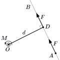 Definition and properties of the moment of force How the moment of force about a fixed axis is calculated
 Project method of coordinates in mathematics and geography Analysis of school textbooks
 A month of assault: why there is no progress seen in the actions of the Western coalition near Mosul All of Iraq is burning