Applications of elementary functions if. Elementary function

1) Function domain and function range.

The domain of a function is the set of all valid valid argument values x(variable x), for which the function y = f(x) determined. The range of a function is the set of all real values y, which the function accepts.

In elementary mathematics, functions are studied only on the set of real numbers.

2) Function zeros.

Function zero is the value of the argument at which the value of the function is equal to zero.

3) Intervals of constant sign of a function.

Intervals of constant sign of a function are sets of argument values on which the function values are only positive or only negative.

4) Monotonicity of the function.

An increasing function (in a certain interval) is a function in which a larger value of the argument from this interval corresponds to a larger value of the function.

A decreasing function (in a certain interval) is a function in which a larger value of the argument from this interval corresponds to a smaller value of the function.

5) Even (odd) function.

An even function is a function whose domain of definition is symmetrical with respect to the origin and for any X from the domain of definition the equality f(-x) = f(x). The graph of an even function is symmetrical about the ordinate.

An odd function is a function whose domain of definition is symmetrical with respect to the origin and for any X from the domain of definition the equality is true f(-x) = - f(x). The graph of an odd function is symmetrical about the origin.

6) Limited and unlimited functions.

A function is called bounded if there is a positive number M such that |f(x)| ≤ M for all values of x. If such a number does not exist, then the function is unlimited.

7) Periodicity of the function.

A function f(x) is periodic if there is a non-zero number T such that for any x from the domain of definition of the function the following holds: f(x+T) = f(x). This smallest number is called the period of the function. All trigonometric functions are periodic. (Trigonometric formulas).

19. Basic elementary functions, their properties and graphs. Application of functions in economics.

Basic elementary functions. Their properties and graphs

1. Linear function.

Linear function is called a function of the form , where x is a variable, a and b are real numbers.

Number A called the slope of the line, it is equal to the tangent of the angle of inclination of this line to the positive direction of the x-axis. The graph of a linear function is a straight line. It is defined by two points.

Properties of a Linear Function

1. Domain of definition - the set of all real numbers: D(y)=R

2. The set of values is the set of all real numbers: E(y)=R

3. The function takes a zero value when or.

4. The function increases (decreases) over the entire domain of definition.

5. A linear function is continuous over the entire domain of definition, differentiable and .

2. Quadratic function.

A function of the form, where x is a variable, coefficients a, b, c are real numbers, is called quadratic

Basic elementary functions, their inherent properties and corresponding graphs are one of the basics of mathematical knowledge, similar in importance to the multiplication table. Elementary functions are the basis, the support for the study of all theoretical issues.

Yandex.RTB R-A-339285-1

The article below provides key material on the topic of basic elementary functions. We will introduce terms, give them definitions; Let's study each type of elementary functions in detail and analyze their properties.

The following types of basic elementary functions are distinguished:

Definition 1

constant function (constant);
nth root;
power function;
exponential function;
logarithmic function;
trigonometric functions;
fraternal trigonometric functions.

A constant function is defined by the formula: y = C (C is a certain real number) and also has a name: constant. This function determines the correspondence of any real value of the independent variable x to the same value of the variable y - the value of C.

The graph of a constant is a straight line that is parallel to the abscissa axis and passes through a point having coordinates (0, C). For clarity, we present graphs of constant functions y = 5, y = - 2, y = 3, y = 3 (indicated in black, red and blue colors in the drawing, respectively).

Definition 2

This elementary function is defined by the formula y = x n (n is a natural number greater than one).

Let's consider two variations of the function.

nth root, n – even number

For clarity, we indicate a drawing that shows graphs of such functions: y = x, y = x 4 and y = x8. These features are color coded: black, red and blue respectively.

The graphs of a function of even degree have a similar appearance for other values of the exponent.

Definition 3

Properties of the nth root function, n is an even number

domain of definition – the set of all non-negative real numbers [ 0 , + ∞) ;
when x = 0, function y = x n has a value equal to zero;
this function is a function of general form (it is neither even nor odd);
range: [ 0 , + ∞) ;
this function y = x n with even root exponents increases throughout the entire domain of definition;
the function has a convexity with an upward direction throughout the entire domain of definition;
there are no inflection points;
there are no asymptotes;
the graph of the function for even n passes through the points (0; 0) and (1; 1).

nth root, n – odd number

Such a function is defined on the entire set of real numbers. For clarity, consider the graphs of the functions y = x 3 , y = x 5 and x 9 . In the drawing they are indicated by colors: black, red and blue are the colors of the curves, respectively.

Other odd values of the root exponent of the function y = x n will give a graph of a similar type.

Definition 4

Properties of the nth root function, n is an odd number

domain of definition – the set of all real numbers;
this function is odd;
range of values – the set of all real numbers;
the function y = x n for odd root exponents increases over the entire domain of definition;
the function has concavity on the interval (- ∞ ; 0 ] and convexity on the interval [ 0 , + ∞);
the inflection point has coordinates (0; 0);
there are no asymptotes;
The graph of the function for odd n passes through the points (- 1 ; - 1), (0 ; 0) and (1 ; 1).

Power function

Definition 5

The power function is defined by the formula y = x a.

The appearance of the graphs and the properties of the function depend on the value of the exponent.

when a power function has an integer exponent a, then the type of graph of the power function and its properties depend on whether the exponent is even or odd, as well as what sign the exponent has. Let's consider all these special cases in more detail below;
the exponent can be fractional or irrational - depending on this, the type of graphs and properties of the function also vary. We will analyze special cases by setting several conditions: 0< a < 1 ; a > 1 ; - 1 < a < 0 и a < - 1 ;
a power function can have a zero exponent; we will also analyze this case in more detail below.

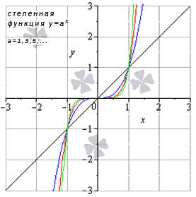
Let's analyze the power function y = x a, when a is an odd positive number, for example, a = 1, 3, 5...

For clarity, we indicate the graphs of such power functions: y = x (graphic color black), y = x 3 (blue color of the graph), y = x 5 (red color of the graph), y = x 7 (graphic color green). When a = 1, we get the linear function y = x.

Definition 6

Properties of a power function when the exponent is odd positive

the function is increasing for x ∈ (- ∞ ; + ∞) ;
the function has convexity for x ∈ (- ∞ ; 0 ] and concavity for x ∈ [ 0 ; + ∞) (excluding the linear function);
the inflection point has coordinates (0 ; 0) (excluding linear function);
there are no asymptotes;
points of passage of the function: (- 1 ; - 1) , (0 ; 0) , (1 ; 1) .

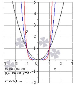
Let's analyze the power function y = x a, when a is an even positive number, for example, a = 2, 4, 6...

For clarity, we indicate the graphs of such power functions: y = x 2 (graphic color black), y = x 4 (blue color of the graph), y = x 8 (red color of the graph). When a = 2, we obtain a quadratic function, the graph of which is a quadratic parabola.

Definition 7

Properties of a power function when the exponent is even positive:

domain of definition: x ∈ (- ∞ ; + ∞) ;
decreasing for x ∈ (- ∞ ; 0 ] ;
the function has concavity for x ∈ (- ∞ ; + ∞) ;
there are no inflection points;
there are no asymptotes;
points of passage of the function: (- 1 ; 1) , (0 ; 0) , (1 ; 1) .

The figure below shows examples of power function graphs y = x a when a is an odd negative number: y = x - 9 (graphic color black); y = x - 5 (blue color of the graph); y = x - 3 (red color of the graph); y = x - 1 (graphic color green). When a = - 1, we obtain inverse proportionality, the graph of which is a hyperbola.

Definition 8

Properties of a power function when the exponent is odd negative:

When x = 0, we obtain a discontinuity of the second kind, since lim x → 0 - 0 x a = - ∞, lim x → 0 + 0 x a = + ∞ for a = - 1, - 3, - 5, …. Thus, the straight line x = 0 is a vertical asymptote;

range: y ∈ (- ∞ ; 0) ∪ (0 ; + ∞) ;
the function is odd because y (- x) = - y (x);
the function is decreasing for x ∈ - ∞ ; 0 ∪ (0 ; + ∞) ;
the function has convexity for x ∈ (- ∞ ; 0) and concavity for x ∈ (0 ; + ∞) ;
there are no inflection points;

k = lim x → ∞ x a x = 0, b = lim x → ∞ (x a - k x) = 0 ⇒ y = k x + b = 0, when a = - 1, - 3, - 5, . . . .

points of passage of the function: (- 1 ; - 1) , (1 ; 1) .

The figure below shows examples of graphs of the power function y = x a when a is an even negative number: y = x - 8 (graphic color black); y = x - 4 (blue color of the graph); y = x - 2 (red color of the graph).

Definition 9

Properties of a power function when the exponent is even negative:

domain of definition: x ∈ (- ∞ ; 0) ∪ (0 ; + ∞) ;

When x = 0, we obtain a discontinuity of the second kind, since lim x → 0 - 0 x a = + ∞, lim x → 0 + 0 x a = + ∞ for a = - 2, - 4, - 6, …. Thus, the straight line x = 0 is a vertical asymptote;

the function is even because y(-x) = y(x);
the function is increasing for x ∈ (- ∞ ; 0) and decreasing for x ∈ 0; + ∞ ;
the function has concavity at x ∈ (- ∞ ; 0) ∪ (0 ; + ∞) ;
there are no inflection points;
horizontal asymptote – straight line y = 0, because:

k = lim x → ∞ x a x = 0 , b = lim x → ∞ (x a - k x) = 0 ⇒ y = k x + b = 0 when a = - 2 , - 4 , - 6 , . . . .

points of passage of the function: (- 1 ; 1) , (1 ; 1) .

From the very beginning, pay attention to the following aspect: in the case when a is a positive fraction with an odd denominator, some authors take the interval - ∞ as the domain of definition of this power function; + ∞ , stipulating that the exponent a is an irreducible fraction. At the moment, the authors of many educational publications on algebra and principles of analysis DO NOT DEFINE power functions, where the exponent is a fraction with an odd denominator for negative values of the argument. Below we will adhere to exactly this position: we will take the set [ 0 ; + ∞) . Recommendation for students: find out the teacher’s view on this point in order to avoid disagreements.

So, let's look at the power function y = x a , when the exponent is a rational or irrational number, provided that 0< a < 1 .

Let us illustrate the power functions with graphs y = x a when a = 11 12 (graphic color black); a = 5 7 (red color of the graph); a = 1 3 (blue color of the graph); a = 2 5 (green color of the graph).

Other values of the exponent a (provided 0< a < 1) дадут аналогичный вид графика.

Definition 10

Properties of the power function at 0< a < 1:

range: y ∈ [ 0 ; + ∞) ;
the function is increasing for x ∈ [ 0 ; + ∞) ;
the function is convex for x ∈ (0 ; + ∞);
there are no inflection points;
there are no asymptotes;

Let's analyze the power function y = x a, when the exponent is a non-integer rational or irrational number, provided that a > 1.

Let us illustrate with graphs the power function y = x a under given conditions using the following functions as an example: y = x 5 4 , y = x 4 3 , y = x 7 3 , y = x 3 π (black, red, blue, green color of the graphs, respectively).

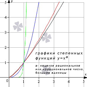
Other values of the exponent a, provided a > 1, will give a similar graph.

Definition 11

Properties of the power function for a > 1:

domain of definition: x ∈ [ 0 ; + ∞) ;
range: y ∈ [ 0 ; + ∞) ;
this function is a function of general form (it is neither odd nor even);
the function is increasing for x ∈ [ 0 ; + ∞) ;
the function has concavity for x ∈ (0 ; + ∞) (when 1< a < 2) и выпуклость при x ∈ [ 0 ; + ∞) (когда a > 2);
there are no inflection points;
there are no asymptotes;
passing points of the function: (0 ; 0) , (1 ; 1) .

Please note! When a is a negative fraction with an odd denominator, in the works of some authors there is an opinion that the domain of definition in this case is the interval - ∞; 0 ∪ (0 ; + ∞) with the caveat that the exponent a is an irreducible fraction. At the moment, the authors of educational materials on algebra and principles of analysis DO NOT DEFINE power functions with an exponent in the form of a fraction with an odd denominator for negative values of the argument. Further, we adhere to exactly this view: we take the set (0 ; + ∞) as the domain of definition of power functions with fractional negative exponents. Recommendation for students: Clarify your teacher's vision at this point to avoid disagreements.

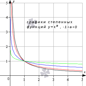
Let's continue the topic and analyze the power function y = x a provided: - 1< a < 0 .

Let us present a drawing of graphs of the following functions: y = x - 5 6, y = x - 2 3, y = x - 1 2 2, y = x - 1 7 (black, red, blue, green color of the lines, respectively).

Definition 12

Properties of the power function at - 1< a < 0:

lim x → 0 + 0 x a = + ∞ when - 1< a < 0 , т.е. х = 0 – вертикальная асимптота;

range: y ∈ 0 ; + ∞ ;
this function is a function of general form (it is neither odd nor even);
there are no inflection points;

The drawing below shows graphs of power functions y = x - 5 4, y = x - 5 3, y = x - 6, y = x - 24 7 (black, red, blue, green colors of the curves, respectively).

Definition 13

Properties of the power function for a< - 1:

domain of definition: x ∈ 0 ; + ∞ ;

lim x → 0 + 0 x a = + ∞ when a< - 1 , т.е. х = 0 – вертикальная асимптота;

range: y ∈ (0 ; + ∞) ;
this function is a function of general form (it is neither odd nor even);
the function is decreasing for x ∈ 0; + ∞ ;
the function has a concavity for x ∈ 0; + ∞ ;
there are no inflection points;
horizontal asymptote – straight line y = 0;
point of passage of the function: (1; 1) .

When a = 0 and x ≠ 0, we obtain the function y = x 0 = 1, which defines the line from which the point (0; 1) is excluded (it was agreed that the expression 0 0 will not be given any meaning).

The exponential function has the form y = a x, where a > 0 and a ≠ 1, and the graph of this function looks different based on the value of the base a. Let's consider special cases.

First, let's look at the situation when the base of the exponential function has a value from zero to one (0< a < 1) . A good example is the graphs of functions for a = 1 2 (blue color of the curve) and a = 5 6 (red color of the curve).

The graphs of the exponential function will have a similar appearance for other values of the base under the condition 0< a < 1 .

Definition 14

Properties of the exponential function when the base is less than one:

range: y ∈ (0 ; + ∞) ;
this function is a function of general form (it is neither odd nor even);
an exponential function whose base is less than one is decreasing over the entire domain of definition;
there are no inflection points;
horizontal asymptote – straight line y = 0 with variable x tending to + ∞;

Now consider the case when the base of the exponential function is greater than one (a > 1).

Let us illustrate this special case with a graph of exponential functions y = 3 2 x (blue color of the curve) and y = e x (red color of the graph).

Other values of the base, larger units, will give a similar appearance to the graph of the exponential function.

Definition 15

Properties of the exponential function when the base is greater than one:

domain of definition – the entire set of real numbers;
range: y ∈ (0 ; + ∞) ;
this function is a function of general form (it is neither odd nor even);
an exponential function whose base is greater than one is increasing as x ∈ - ∞; + ∞ ;
the function has a concavity at x ∈ - ∞; + ∞ ;
there are no inflection points;
horizontal asymptote – straight line y = 0 with variable x tending to - ∞;
point of passage of the function: (0; 1) .

The logarithmic function has the form y = log a (x), where a > 0, a ≠ 1.

Such a function is defined only for positive values of the argument: for x ∈ 0; + ∞ .

The graph of a logarithmic function has a different appearance, based on the value of the base a.

Let us first consider the situation when 0< a < 1 . Продемонстрируем этот частный случай графиком логарифмической функции при a = 1 2 (синий цвет кривой) и а = 5 6 (красный цвет кривой).

Other values of the base, not larger units, will give a similar type of graph.

Definition 16

Properties of a logarithmic function when the base is less than one:

domain of definition: x ∈ 0 ; + ∞ . As x tends to zero from the right, the function values tend to +∞;
range of values: y ∈ - ∞ ; + ∞ ;
this function is a function of general form (it is neither odd nor even);
logarithmic
the function has a concavity for x ∈ 0; + ∞ ;
there are no inflection points;
there are no asymptotes;

Now let's look at the special case when the base of the logarithmic function is greater than one: a > 1 . The drawing below shows graphs of logarithmic functions y = log 3 2 x and y = ln x (blue and red colors of the graphs, respectively).

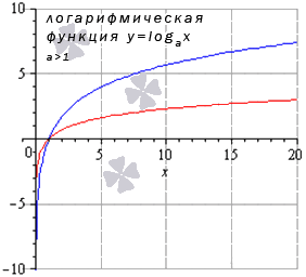
Other values of the base greater than one will give a similar type of graph.

Definition 17

Properties of a logarithmic function when the base is greater than one:

domain of definition: x ∈ 0 ; + ∞ . As x tends to zero from the right, the function values tend to - ∞ ;
range of values: y ∈ - ∞ ; + ∞ (the entire set of real numbers);
this function is a function of general form (it is neither odd nor even);
the logarithmic function is increasing for x ∈ 0; + ∞ ;
the function is convex for x ∈ 0; + ∞ ;
there are no inflection points;
there are no asymptotes;
point of passage of the function: (1; 0) .

The trigonometric functions are sine, cosine, tangent and cotangent. Let's look at the properties of each of them and the corresponding graphics.

In general, all trigonometric functions are characterized by the property of periodicity, i.e. when the values of the functions are repeated for different values of the argument, differing from each other by the period f (x + T) = f (x) (T is the period). Thus, the item “smallest positive period” is added to the list of properties of trigonometric functions. In addition, we will indicate the values of the argument at which the corresponding function becomes zero.

Sine function: y = sin(x)

The graph of this function is called a sine wave.

Definition 18

Properties of the sine function:

domain of definition: the entire set of real numbers x ∈ - ∞ ; + ∞ ;
the function vanishes when x = π · k, where k ∈ Z (Z is the set of integers);
the function is increasing for x ∈ - π 2 + 2 π · k ; π 2 + 2 π · k, k ∈ Z and decreasing for x ∈ π 2 + 2 π · k; 3 π 2 + 2 π · k, k ∈ Z;
the sine function has local maxima at points π 2 + 2 π · k; 1 and local minima at points - π 2 + 2 π · k; - 1, k ∈ Z;
the sine function is concave when x ∈ - π + 2 π · k ; 2 π · k, k ∈ Z and convex when x ∈ 2 π · k; π + 2 π k, k ∈ Z;
there are no asymptotes.

Cosine function: y = cos(x)

The graph of this function is called a cosine wave.

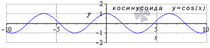
Definition 19

Properties of the cosine function:

domain of definition: x ∈ - ∞ ; + ∞ ;
smallest positive period: T = 2 π;
range of values: y ∈ - 1 ; 1 ;
this function is even, since y (- x) = y (x);
the function is increasing for x ∈ - π + 2 π · k ; 2 π · k, k ∈ Z and decreasing for x ∈ 2 π · k; π + 2 π k, k ∈ Z;
the cosine function has local maxima at points 2 π · k ; 1, k ∈ Z and local minima at points π + 2 π · k; - 1, k ∈ z;
the cosine function is concave when x ∈ π 2 + 2 π · k ; 3 π 2 + 2 π · k , k ∈ Z and convex when x ∈ - π 2 + 2 π · k ; π 2 + 2 π · k, k ∈ Z;
inflection points have coordinates π 2 + π · k; 0 , k ∈ Z
there are no asymptotes.

Tangent function: y = t g (x)

The graph of this function is called tangent.

Definition 20

Properties of the tangent function:

domain of definition: x ∈ - π 2 + π · k ; π 2 + π · k, where k ∈ Z (Z is the set of integers);
Behavior of the tangent function on the boundary of the domain of definition lim x → π 2 + π · k + 0 t g (x) = - ∞ , lim x → π 2 + π · k - 0 t g (x) = + ∞ . Thus, the straight lines x = π 2 + π · k k ∈ Z are vertical asymptotes;
the function vanishes when x = π · k for k ∈ Z (Z is the set of integers);
range of values: y ∈ - ∞ ; + ∞ ;
this function is odd, since y (- x) = - y (x) ;
the function is increasing as - π 2 + π · k ; π 2 + π · k, k ∈ Z;
the tangent function is concave for x ∈ [π · k; π 2 + π · k) , k ∈ Z and convex for x ∈ (- π 2 + π · k ; π · k ] , k ∈ Z ;
inflection points have coordinates π · k ; 0 , k ∈ Z ;

Cotangent function: y = c t g (x)

The graph of this function is called a cotangentoid. .

Definition 21

Properties of the cotangent function:

domain of definition: x ∈ (π · k ; π + π · k) , where k ∈ Z (Z is the set of integers);

Behavior of the cotangent function on the boundary of the domain of definition lim x → π · k + 0 t g (x) = + ∞ , lim x → π · k - 0 t g (x) = - ∞ . Thus, the straight lines x = π · k k ∈ Z are vertical asymptotes;

smallest positive period: T = π;
the function vanishes when x = π 2 + π · k for k ∈ Z (Z is the set of integers);
range of values: y ∈ - ∞ ; + ∞ ;
this function is odd, since y (- x) = - y (x) ;
the function is decreasing for x ∈ π · k ; π + π k, k ∈ Z;
the cotangent function is concave for x ∈ (π · k; π 2 + π · k ], k ∈ Z and convex for x ∈ [ - π 2 + π · k ; π · k), k ∈ Z ;
inflection points have coordinates π 2 + π · k; 0 , k ∈ Z ;
There are no oblique or horizontal asymptotes.

The inverse trigonometric functions are arcsine, arccosine, arctangent and arccotangent. Often, due to the presence of the prefix “arc” in the name, inverse trigonometric functions are called arc functions .

Arc sine function: y = a r c sin (x)

Definition 22

Properties of the arcsine function:

this function is odd, since y (- x) = - y (x) ;
the arcsine function has a concavity for x ∈ 0; 1 and convexity for x ∈ - 1 ; 0 ;
inflection points have coordinates (0; 0), which is also the zero of the function;
there are no asymptotes.

Arc cosine function: y = a r c cos (x)

Definition 23

Properties of the arc cosine function:

domain of definition: x ∈ - 1 ; 1 ;
range: y ∈ 0 ; π;
this function is of a general form (neither even nor odd);
the function is decreasing over the entire domain of definition;
the arc cosine function has a concavity at x ∈ - 1; 0 and convexity for x ∈ 0; 1 ;
inflection points have coordinates 0; π 2;
there are no asymptotes.

Arctangent function: y = a r c t g (x)

Definition 24

Properties of the arctangent function:

domain of definition: x ∈ - ∞ ; + ∞ ;
range of values: y ∈ - π 2 ; π 2;
this function is odd, since y (- x) = - y (x) ;
the function is increasing over the entire domain of definition;
the arctangent function has concavity for x ∈ (- ∞ ; 0 ] and convexity for x ∈ [ 0 ; + ∞);
the inflection point has coordinates (0; 0), which is also the zero of the function;
horizontal asymptotes are straight lines y = - π 2 as x → - ∞ and y = π 2 as x → + ∞ (in the figure, the asymptotes are green lines).

Arc tangent function: y = a r c c t g (x)

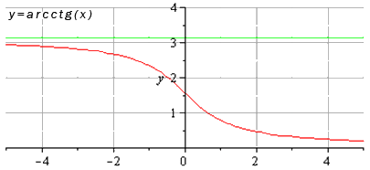
Definition 25

Properties of the arccotangent function:

domain of definition: x ∈ - ∞ ; + ∞ ;
range: y ∈ (0; π) ;
this function is of a general form;
the function is decreasing over the entire domain of definition;
the arc cotangent function has a concavity for x ∈ [ 0 ; + ∞) and convexity for x ∈ (- ∞ ; 0 ] ;
the inflection point has coordinates 0; π 2;
horizontal asymptotes are straight lines y = π at x → - ∞ (green line in the drawing) and y = 0 at x → + ∞.

If you notice an error in the text, please highlight it and press Ctrl+Enter

Complete list of basic elementary functions

The class of basic elementary functions includes the following:

Constant function $y=C$, where $C$ is a constant. Such a function takes the same value $C$ for any $x$.
Power function $y=x^(a) $, where the exponent $a$ is a real number.
Exponential function $y=a^(x) $, where the base is degree $a>0$, $a\ne 1$.
Logarithmic function $y=\log _(a) x$, where the base of the logarithm is $a>0$, $a\ne 1$.
Trigonometric functions $y=\sin x$, $y=\cos x$, $y=tg\, x$, $y=ctg\, x$, $y=\sec x$, $y=A>\ sec\,x$.
Inverse trigonometric functions $y=\arcsin x$, $y=\arccos x$, $y=arctgx$, $y=arcctgx$, $y=arc\sec x$, $y=arc\, \cos ec\ , x$.

Power functions

We will consider the behavior of the power function $y=x^(a) $ for those simplest cases when its exponent determines integer exponentiation and root extraction.

Case 1

The exponent of the function $y=x^(a) $ is a natural number, that is, $y=x^(n) $, $n\in N$.

If $n=2\cdot k$ is an even number, then the function $y=x^(2\cdot k) $ is even and increases indefinitely as if the argument $\left(x\to +\infty \ right)$, and with its unlimited decrease $\left(x\to -\infty \right)$. This behavior of the function can be described by the expressions $\mathop(\lim )\limits_(x\to +\infty ) x^(2\cdot k) =+\infty $ and $\mathop(\lim )\limits_(x\to -\infty ) x^(2\cdot k) =+\infty $, which mean that the function in both cases increases without limit ($\lim $ is the limit). Example: graph of the function $y=x^(2) $.

If $n=2\cdot k-1$ is an odd number, then the function $y=x^(2\cdot k-1) $ is odd, increases indefinitely as the argument increases indefinitely, and decreases indefinitely as the argument decreases indefinitely. This behavior of the function can be described by the expressions $\mathop(\lim )\limits_(x\to +\infty ) x^(2\cdot k-1) =+\infty $ and $\mathop(\lim )\limits_(x \to -\infty ) x^(2\cdot k-1) =-\infty $. Example: graph of the function $y=x^(3) $.

Case 2

The exponent of the function $y=x^(a) $ is a negative integer, that is, $y=\frac(1)(x^(n) ) $, $n\in N$.

If $n=2\cdot k$ is an even number, then the function $y=\frac(1)(x^(2\cdot k) ) $ is even and asymptotically (gradually) approaches zero as with unlimited increase argument, and with its unlimited decrease. This behavior of the function can be described by a single expression $\mathop(\lim )\limits_(x\to \infty ) \frac(1)(x^(2\cdot k) ) =0$, which means that with an unlimited increase in the argument in absolute value, the limit of the function is zero. In addition, as the argument tends to zero both on the left $\left(x\to 0-0\right)$ and on the right $\left(x\to 0+0\right)$, the function increases without limit. Therefore, the expressions $\mathop(\lim )\limits_(x\to 0-0) \frac(1)(x^(2\cdot k) ) =+\infty $ and $\mathop(\lim )\limits_ are valid (x\to 0+0) \frac(1)(x^(2\cdot k) ) =+\infty $, which means that the function $y=\frac(1)(x^(2\cdot k ) ) $ in both cases has an infinite limit equal to $+\infty $. Example: graph of the function $y=\frac(1)(x^(2) ) $.

If $n=2\cdot k-1$ is an odd number, then the function $y=\frac(1)(x^(2\cdot k-1) ) $ is odd and asymptotically approaches zero as if both when the argument increases and when it decreases without limit. This behavior of the function can be described by a single expression $\mathop(\lim )\limits_(x\to \infty ) \frac(1)(x^(2\cdot k-1) ) =0$. In addition, as the argument approaches zero on the left, the function decreases without limit, and as the argument approaches zero on the right, the function increases without limit, that is, $\mathop(\lim )\limits_(x\to 0-0) \frac(1)(x ^(2\cdot k-1) ) =-\infty $ and $\mathop(\lim )\limits_(x\to 0+0) \frac(1)(x^(2\cdot k-1) ) =+\infty $. Example: graph of the function $y=\frac(1)(x) $.

Case 3

The exponent of the function $y=x^(a) $ is the inverse of the natural number, that is, $y=\sqrt[(n)](x) $, $n\in N$.

If $n=2\cdot k$ is an even number, then the function $y=\pm \sqrt[(2\cdot k)](x) $ is two-valued and is defined only for $x\ge 0$. With an unlimited increase in the argument, the value of the function $y=+\sqrt[(2\cdot k)](x) $ increases unlimitedly, and the value of the function $y=-\sqrt[(2\cdot k)](x) $ decreases unlimitedly , that is, $\mathop(\lim )\limits_(x\to +\infty ) \left(+\sqrt[(2\cdot k)](x) \right)=+\infty $ and $\mathop( \lim )\limits_(x\to +\infty ) \left(-\sqrt[(2\cdot k)](x) \right)=-\infty $. Example: graph of the function $y=\pm \sqrt(x) $.

If $n=2\cdot k-1$ is an odd number, then the function $y=\sqrt[(2\cdot k-1)](x) $ is odd, increases unlimitedly with an unlimited increase in the argument and decreases unlimitedly when unlimited, it decreases, that is, $\mathop(\lim )\limits_(x\to +\infty ) \sqrt[(2\cdot k-1)](x) =+\infty $ and $\mathop(\ lim )\limits_(x\to -\infty ) \sqrt[(2\cdot k-1)](x) =-\infty $. Example: graph of the function $y=\sqrt[(3)](x) $.

Exponential and logarithmic functions

The exponential $y=a^(x) $ and logarithmic $y=\log _(a) x$ functions are mutually inverse. Their graphs are symmetrical with respect to the common bisector of the first and third coordinate angles.

As the argument $\left(x\to +\infty \right)$ increases indefinitely, the exponential function or $\mathop(\lim )\limits_(x\to +\infty ) a^(x) =+\infty $ increases indefinitely , if $a>1$, or asymptotically approaches zero $\mathop(\lim )\limits_(x\to +\infty ) a^(x) =0$, if $a1$, or $\mathop increases without limit (\lim )\limits_(x\to -\infty ) a^(x) =+\infty $, if $a

The characteristic value for the function $y=a^(x) $ is the value $x=0$. In this case, all exponential functions, regardless of $a$, necessarily intersect the $Oy$ axis at $y=1$. Examples: graphs of the functions $y=2^(x) $ and $y = \left (\frac(1)(2) \right)^(x) $.

The logarithmic function $y=\log _(a) x$ is defined only for $x > 0$.

As the argument $\left(x\to +\infty \right)$ increases indefinitely, the logarithmic function or $\mathop(\lim )\limits_(x\to +\infty ) \log _(a) x=+\ increases indefinitely infty $, if $a>1$, or decreases without limit $\mathop(\lim )\limits_(x\to +\infty ) \log _(a) x=-\infty $, if $a1$, or without limit $\mathop(\lim )\limits_(x\to 0+0) \log _(a) x=+\infty $ increases if $a

The characteristic value for the function $y=\log _(a) x$ is the value $y=0$. In this case, all logarithmic functions, regardless of $a$, necessarily intersect the $Ox$ axis at $x=1$. Examples: graphs of the functions $y=\log _(2) x$ and $y=\log _(1/2) x$.

Some logarithmic functions have special notation. In particular, if the base of the logarithm is $a=10$, then such a logarithm is called decimal, and the corresponding function is written as $y=\lg x$. And if the irrational number $e=2.7182818\ldots $ is chosen as the base of the logarithm, then such a logarithm is called natural, and the corresponding function is written as $y=\ln x$. Its inverse is the function $y=e^(x) $, called the exponent.

The section contains reference material on the main elementary functions and their properties. A classification of elementary functions is given. Below are links to subsections that discuss the properties of specific functions - graphs, formulas, derivatives, antiderivatives (integrals), series expansions, expressions through complex variables.

Content

Reference pages for basic functions

Classification of elementary functions

Algebraic function is a function that satisfies the equation:
,
where is a polynomial in the dependent variable y and the independent variable x. It can be written as:
,
where are polynomials.

Algebraic functions are divided into polynomials (entire rational functions), rational functions and irrational functions.

Entire rational function, which is also called polynomial or polynomial, is obtained from the variable x and a finite number of numbers using the arithmetic operations of addition (subtraction) and multiplication. After opening the brackets, the polynomial is reduced to canonical form:
.

Fractional rational function, or simply rational function, is obtained from the variable x and a finite number of numbers using the arithmetic operations of addition (subtraction), multiplication and division. The rational function can be reduced to the form
,
where and are polynomials.

Irrational function is an algebraic function that is not rational. As a rule, an irrational function is understood as roots and their compositions with rational functions. A root of degree n is defined as the solution to the equation
.
It is designated as follows:
.

Transcendental functions are called non-algebraic functions. These are exponential, trigonometric, hyperbolic and their inverse functions.

Overview of basic elementary functions

All elementary functions can be represented as a finite number of addition, subtraction, multiplication and division operations performed on an expression of the form:
z t .
Inverse functions can also be expressed in terms of logarithms. The basic elementary functions are listed below.

Power function :
y(x) = xp,
where p is the exponent. It depends on the base of the degree x.
The inverse of the power function is also the power function:
.
For an integer non-negative value of the exponent p, it is a polynomial. For an integer value p - a rational function. With a rational meaning - an irrational function.

Transcendental functions

Exponential function :
y(x) = a x ,
where a is the base of the degree. It depends on the exponent x.
The inverse function is the logarithm to base a:
x = log a y.

Exponent, e to the x power:
y(x) = e x ,
This is an exponential function whose derivative is equal to the function itself:
.
The base of the exponent is the number e:
≈ 2,718281828459045... .
The inverse function is the natural logarithm - the logarithm to the base of the number e:
x = ln y ≡ log e y.

Trigonometric functions:
Sine: ;
Cosine: ;
Tangent: ;
Cotangent: ;
Here i is the imaginary unit, i 2 = -1.

Inverse trigonometric functions:
Arcsine: x = arcsin y, ;
Arc cosine: x = arccos y, ;
Arctangent: x = arctan y, ;
Arc tangent: x = arcctg y, .