Types of matrices. Stepwise Matrix View

ODA. Rectangular table with t lines and P columns of real numbers is called matrix size t×n. Matrices are denoted by capital Latin letters: A, B, ..., and an array of numbers is distinguished by round or square brackets.

The numbers included in the table are called matrix elements and are denoted by small Latin letters with a double index, where i- line number j– number of the column at the intersection of which the element is located. In general, the matrix is written as follows:

Two matrices are considered equal if their corresponding elements are equal.

If the number of matrix rows t equal to the number of its columns P, then the matrix is called square(otherwise rectangular).

Size Matrix
is called a row matrix. Size Matrix

is called a column matrix.

Matrix elements with equal indices (
etc.), form main diagonal matrices. The other diagonal is called the side diagonal.

The square matrix is called diagonal if all its elements located outside the main diagonal are equal to zero.

A diagonal matrix whose diagonal entries are equal to one is called single matrix and has the standard notation E:

If all elements of a matrix located above (or below) the main diagonal are equal to zero, the matrix is said to have a triangular form:

§2. Matrix operations

1. Matrix transposition - a transformation in which the rows of the matrix are written as columns while maintaining their order. For a square matrix, this transformation is equivalent to a symmetric mapping with respect to the main diagonal:

2. Matrices of the same dimension can be summed (subtracted). The sum (difference) of matrices is a matrix of the same dimension, each element of which is equal to the sum (difference) of the corresponding elements of the original matrices:

3. Any matrix can be multiplied by a number. The product of a matrix by a number is a matrix of the same order, each element of which is equal to the product of the corresponding element of the original matrix by this number:

4. If the number of columns of one matrix is equal to the number of rows of another, then you can multiply the first matrix by the second. The product of such matrices is a matrix, each element of which is equal to the sum of pairwise products of the elements of the corresponding row of the first matrix and the elements of the corresponding column of the second matrix.

Consequence. Matrix exponentiation to>1 is the product of the matrix A to once. Defined for square matrices only.

Example.

Properties of operations on matrices.

(A+B)+C=A+(B+C);
k(A+B)=kA+kV;
A(B+C)=AB+AC;
(A+B)C=AC+BC;
k(AB)=(kA)B=A(kV);
A(BC)=(AB)C;
(kA) T =kA T;
(A + B) T \u003d A T + B T;
(AB) T =B T A T;

The properties listed above are similar to the properties of operations on numbers. There are also specific properties of matrices. These include, for example, the distinctive property of matrix multiplication. If the product AB exists, then the product BA

Might not exist

May differ from AB.

Example. The company manufactures products of two types A and B and uses three types of raw materials S 1 , S 2 , and S 3 . The consumption rates of raw materials are given by the matrix N=
, where n ij- quantity of raw materials j spent on the production of a unit of output i. The production plan is given by the matrix C = (100 200), and the unit cost of each type of raw material is given by the matrix . Determine the cost of raw materials required for the planned output and the total cost of raw materials.

Solution. The cost of raw materials is defined as the product of matrices C and N:

We calculate the total cost of raw materials as the product of S and P.

A matrix is a rectangular table of numbers, consisting of m strings of the same length or n columns of the same length.

aij- element of the matrix, which is in i -th line and j -th column.

For brevity, the matrix can be denoted by a single capital letter, for example, BUT or AT.

In general, a matrix of size m× n write like this

Examples:

If the number of rows in a matrix is equal to the number of columns, then the matrix is called square, and the number of its rows or columns is called in order matrices. In the examples above, the second matrix is square - its order is 3, and the fourth matrix - its order is 1.

A matrix in which the number of rows is not equal to the number of columns is called rectangular. In the examples, this is the first matrix and the third.

main diagonal A square matrix is the diagonal going from the upper left to the lower right corner.

A square matrix in which all elements below the main diagonal are equal to zero is called triangular matrix.

A square matrix in which all elements, except perhaps those on the main diagonal, are equal to zero, is called diagonal matrix. For example, or.

A diagonal matrix in which all diagonal entries are equal to one is called single matrix and is denoted by the letter E. For example, the 3rd order identity matrix has the form .

back to content

(36)85. What are linear operations on matrices? Examples.

In all cases when new mathematical objects are introduced, it is necessary to agree on the rules of action on them, and also to determine which objects are considered equal to each other.

The nature of the objects is irrelevant. It can be real or complex numbers, vectors, matrices, strings, or something else.

The standard operations include linear operations, namely: multiplication by a number and addition; in this particular case - multiplication of matrices by a number and addition of matrices.

When multiplying a matrix by a number, each matrix element is multiplied by that number, and matrix addition implies pairwise addition of elements located in equivalent positions.

Terminological expression "linear combination<" (векторов, матриц, строк, столбцов и так далее) всегда означает одно и тоже: алгебраическая сумма этих векторов (или матриц, строк, столбцов и так далее), предварительно умноженных на числовые коэффициенты.

matrices A = || a i j|| and B = || a i j|| are considered equal if they have the same dimensions and their corresponding matrix elements are pairwise equal:

Matrix addition The addition operation is only defined for matrices of the same size. The result of matrix addition A = || a i j|| and B = || b i j|| is the matrix C = || c i j|| , whose elements are equal to the sum of the corresponding matrix elements.

The matrix is denoted by capital Latin letters ( BUT, AT, FROM,...).

Definition 1. Rectangular table of the form ,

consisting of m lines and n columns is called matrix.

Matrix element, i – row number, j – column number.

Types of matrices:

elements on the main diagonal:

trA=a 11 +a 22 +a 33 +…+a nn .

§2. Determinants of 2nd, 3rd and nth order

Let two square matrices be given:

Definition 1. Determinant of the second order of a matrix BUT 1 is the number denoted by ∆ and equal to , where

Example. Calculate the 2nd order determinant:

Definition 2. Determinant of the 3rd order of a square matrix BUT 2 called a number of the form:

This is one way to calculate the determinant.

Example. Calculate

Definition 3. If a determinant consists of n-rows and n-columns, then it is called an n-th order determinant.

Properties of determinants:

The determinant does not change during transposition (i.e., if the rows and columns in it are interchanged while maintaining the order).

If any two rows or two columns are interchanged in the determinant, then the determinant only changes the sign.

The common factor of any row (column) can be taken out of the sign of the determinant.

If all elements of any row (column) of the determinant are equal to zero, then the determinant is equal to zero.

The determinant is zero if the elements of any two rows are equal or proportional.

The determinant does not change if the corresponding elements of another row (column) multiplied by the same number are added to the elements of any row (column).

Example.

Definition 4. The determinant obtained from a given by deleting a column and a row is called minor the corresponding element. M ij element a ij .

Definition 5. Algebraic addition element a ij , is called the expression

§3. Matrix Actions

Linear operations

1) When adding matrices, their elements of the same name are added.

When subtracting matrices, their elements of the same name are subtracted.

When multiplying a matrix by a number, each element of the matrix is multiplied by that number:

3.2 Matrix multiplication.

Work matrices BUT to matrix AT is a new matrix whose elements are equal to the sum of the products of the elements of the i-th row of the matrix BUT to the corresponding elements of the jth column of the matrix AT. Matrix product BUT to matrix AT can only be found if the number of columns of the matrix BUT equals the number of matrix rows AT. Otherwise, the work is impossible.

Comment:

(not subject to the commutativity property)

§ 4. Inverse matrix

The inverse matrix exists only for a square matrix, and the matrix must be nonsingular.

Definition 1. Matrix BUT called non-degenerate if the determinant of this matrix is not equal to zero

Definition 2. BUT-1 called inverse matrix for a given non-singular square matrix BUT, if when multiplying this matrix by the given one both on the right, then on the left, the identity matrix is obtained.

Algorithm for calculating the inverse matrix

1 way (using algebraic additions)

Example 1:

Matrices. Types of matrices. Operations on matrices and their properties.

Determinant of the matrix of the nth order. N, Z, Q, R, C,

A matrix of order m*n is a rectangular table of numbers containing m-rows and n-columns.

Matrix equality:

Two matrices are called equal if the number of rows and columns of one of them is equal, respectively, to the number of rows and columns of the other and, respectively. the elements of these matrices are equal.

Note: Elements with the same indexes are matched.

Types of matrices:

Square Matrix: A matrix is said to be square if the number of rows is equal to the number of columns.

Rectangular: A matrix is said to be rectangular if the number of rows is not equal to the number of columns.

Row matrix: a matrix of order 1*n (m=1) has the form a11,a12,a13 and is called a row matrix.

Matrix column:………….

Diagonal: the diagonal of a square matrix, going from the upper left corner to the lower right corner, that is, consisting of elements a11, a22 ...... - is called the main diagonal. (definition: a square matrix, all elements of which are equal to zero, except for those located on the main diagonal, is called a diagonal matrix.

Identity: A diagonal matrix is called identity if all elements are located on the main diagonal and are equal to 1.

Upper triangular: A=||aij|| is called an upper triangular matrix if aij=0. Provided i>j.

Lower triangular: aij=0. i

Zero: This is a matrix whose Els are 0.

Operations on matrices.

1. Transposition.

2. Multiplication of a matrix by a number.

3. Matrix addition.

4. Matrix multiplication.

Basic sv-va action on matrices.

1.A+B=B+A (commutativity)

2.A+(B+C)=(A+B)+C (associativity)

3.a(A+B)=aA+aB (distributivity)

4.(a+b)A=aA+bA (distributive)

5.(ab)A=a(bA)=b(aA) (asoots.)

6.AB≠BA (no commu.)

7.A(BC)=(AB)C (associative) – executed if def. Matrix products are performed.

8.A(B+C)=AB+AC (distributive)

(B+C)A=BA+CA (distributive)

9.a(AB)=(aA)B=(aB)A

Determinant of a square matrix - definition and its properties. Decomposition of the determinant in rows and columns. Methods for calculating determinants.

If matrix A has order m>1, then the determinant of this matrix is a number.

The algebraic complement Aij of the element aij of matrix A is the minor Mij multiplied by the number

THEOREM1: The determinant of the matrix A is equal to the sum of the products of all elements of an arbitrary row (column) and their algebraic complements.

Basic properties of determinants.

1. The determinant of a matrix will not change when it is transposed.

2. When permuting two rows (columns), the determinant changes sign, but its absolute value does not change.

3. The determinant of a matrix that has two identical rows (columns) is 0.

4. When multiplying a row (column) of a matrix by a number, its determinant is multiplied by this number.

5. If one of the rows (columns) of the matrix consists of 0, then the determinant of this matrix is 0.

6. If all elements of the i-th row (column) of a matrix are presented as a sum of two terms, then its determinant can be represented as a sum of determinants of two matrices.

7. The determinant will not change if, respectively, the elements of one column (row) are added to the elements of another column (row) by premultiplying. for the same number.

8. The sum of arbitrary elements of any column (row) of the determinant to the corresponding algebraic complement of elements of another column (row) is 0.

https://pandia.ru/text/78/365/images/image004_81.gif" width="46" height="27">

Methods for calculating the determinant:

1. By definition or Theorem 1.

2. Reduction to a triangular form.

Definition and properties of the inverse matrix. Calculation of the inverse matrix. Matrix equations.

Definition: A square matrix of order n is called the inverse of a matrix A of the same order and is denoted

In order for the matrix A to have an inverse matrix, it is necessary and sufficient that the determinant of the matrix A is different from 0.

Inverse Matrix Properties:

1. Uniqueness: for a given matrix A, its inverse is unique.

2. matrix determinant

3. The operation of taking the transposition and taking the inverse matrix.

Matrix equations:

Let A and B be two square matrices of the same order.

https://pandia.ru/text/78/365/images/image008_56.gif" width="163" height="11 src=">

The concept of linear dependence and independence of matrix columns. Properties of linear dependence and linear independence of the column system.

Columns А1,А2…An are called linearly dependent if there is a non-trivial linear combination of them equal to the 0th column.

Columns А1,А2…An are called linearly independent if there is a non-trivial linear combination of them equal to the 0th column.

A linear combination is called trivial if all coefficients С(l) are equal to 0 and non-trivial otherwise.

https://pandia.ru/text/78/365/images/image010_52.gif" width="88" height="24">

2. In order for the columns to be linearly dependent, it is necessary and sufficient that some column be a linear combination of other columns.

Let 1 of the columns https://pandia.ru/text/78/365/images/image014_42.gif" width="13" height="23 src="> be a linear combination of other columns.

https://pandia.ru/text/78/365/images/image016_38.gif" width="79" height="24"> are linearly dependent, then all columns are linearly dependent.

4. If a system of columns is linearly independent, then any of its subsystems is also linearly independent.

(Everything that is said about columns is also true for rows).

Matrix minors. Basis minors. Matrix rank. The method of fringing minors for calculating the rank of a matrix.

The order minor of matrix A is the determinant whose elements are located at the intersection of k-rows and k-rows of matrix A.

If all minors of order k of the matrix A = 0, then any minor of order k + 1 is also equal to 0.

Basic minor.

The rank of a matrix A is the order of its basis minor.

The method of bordering minors: - We choose a non-zero element of the matrix A (If such an element does not exist, then the rank of A \u003d 0)

We border the previous minor of the 1st order with the minor of the 2nd order. (If this minor is not equal to 0, then the rank >=2) If the rank of this minor =0, then we border the chosen 1st order minor with other 2nd order minors. (If all minors of the 2nd order = 0, then the rank of the matrix = 1).

Matrix rank. Methods for finding the rank of a matrix.

The rank of a matrix A is the order of its basis minor.

Calculation methods:

1) The method of bordering minors: -Choose a non-zero element of the matrix A (if there is no such element, then rank = 0) - Border the previous 1st order minor with the 2nd order minor..gif" width="40" height="22" >r+1 Mr+1=0.

2) Bringing a matrix to a stepped form: this method is based on elementary transformations. Under elementary transformations, the rank of the matrix does not change.

The following transformations are called elementary transformations:

Permutation of two rows (columns).

Multiplication of all elements of some column (row) by a number not =0.

Addition to all elements of a certain column (row) of elements of another column (row), previously multiplied by the same number.

Basis minor theorem. Necessary and sufficient condition for the determinant to be equal to zero.

The basis minor of the matrix A is the minor of the largest k-th order different from 0.

Basis minor theorem:

Basic rows (columns) are linearly independent. Any row (column) of matrix A is a linear combination of basic rows (columns).

Notes: Rows and columns at the intersection of which there is a basic minor are called basic rows and columns, respectively.

a11 a12… a1r a1j

a21 a22….a2r a2j

a31 a32….a3r a3j

ar1 ar2 ….arr arj

ak1 ak2…..akr akj

Necessary and sufficient conditions for the determinant to be equal to zero:

In order for the determinant of the nth order = 0, it is necessary and sufficient that its rows (columns) be linearly dependent.

Systems of linear equations, their classification and notation forms. Cramer's rule.

Consider a system of 3 linear equations with three unknowns:

https://pandia.ru/text/78/365/images/image020_29.gif" alt="(!LANG:l14image048" width="64" height="38 id=">!}

is called the determinant of the system.

We compose three more determinants as follows: we replace successively 1, 2 and 3 columns in the determinant D with a column of free terms

https://pandia.ru/text/78/365/images/image022_23.gif" alt="(!LANG:l14image052" width="93" height="22 id=">!}

Proof. So, consider a system of 3 equations with three unknowns. We multiply the 1st equation of the system by the algebraic complement A11 of the element a11, the 2nd equation by A21 and the 3rd one by A31:

https://pandia.ru/text/78/365/images/image024_24.gif" alt="(!LANG:l14image056" width="247" height="31 id=">!}

Consider each of the brackets and the right side of this equation. By the theorem on the expansion of the determinant in terms of the elements of the 1st column

https://pandia.ru/text/78/365/images/image026_23.gif" alt="(!LANG:l14image060" width="324" height="42 id=">!}

Similarly, it can be shown that and .

Finally, it is easy to see that

Thus, we get the equality: .

Consequently, .

The equalities and are derived similarly, whence the assertion of the theorem follows.

Systems of linear equations. Compatibility condition for linear equations. The Kronecker-Capelli theorem.

The solution of a system of algebraic equations is such a set of n numbers C1,C2,C3……Cn, which, when substituted into the original system in place of x1,x2,x3…..xn, turns all the equations of the system into identities.

A system of linear algebraic equations is called consistent if it has at least one solution.

A joint system is called definite if it has a unique solution, and indefinite if it has infinitely many solutions.

Conditions for the compatibility of systems of linear algebraic equations.

a11 a12 ……a1n x1 b1

a21 a22 ……a2n x2 b2

……………….. .. = ..

am1 am2…..amn xn bn

THEOREM: For a system of m linear equations with n unknowns to be consistent, it is necessary and sufficient that the rank of the extended matrix be equal to the rank of matrix A.

Note: This theorem only gives criteria for the existence of a solution, but does not indicate a way to find a solution.

10 question.

Systems of linear equations. The basis minor method is a general method for finding all solutions to systems of linear equations.

A=a21 a22…..a2n

Basis minor method:

Let the system be consistent and RgA=RgA’=r. Let the basic minor be painted in the upper left corner of the matrix A.

https://pandia.ru/text/78/365/images/image035_20.gif" width="22" height="23 src=">…...gif" width="23" height="23 src= ">…...gif" width="22" height="23 src=">…...gif" width="46" height="23 src=">-…..-a

d2 b2-a(2r+1)x(r+1)-..-a(2n)x(n)

… = …………..

Dr br-a(rr+1)x(r+1)-..-a(rn)x(n)

https://pandia.ru/text/78/365/images/image050_12.gif" width="33" height="22 src=">

Remarks: If the rank of the main matrix and considered is equal to r=n, then in this case dj=bj and the system has a unique solution.

Homogeneous systems of linear equations.

A system of linear algebraic equations is called homogeneous if all its free terms are equal to zero.

AX=0 is a homogeneous system.

AX = B is an inhomogeneous system.

Homogeneous systems are always compatible.

X1 =x2 =..=xn =0

Theorem 1.

Homogeneous systems have non-homogeneous solutions when the rank of the system matrix is less than the number of unknowns.

Theorem 2.

A homogeneous system of n-linear equations with n-unknowns has a non-zero solution when the determinant of the matrix A is equal to zero. (detA=0)

Properties of solutions of homogeneous systems.

Any linear combination of a solution to a homogeneous system is itself a solution to this system.

α1C1 +α2C2 ; α1 and α2 are some numbers.

A(α1C1 + α2C2) = A(α1C1) + A(α2C2) = α1(A C1) + α2(AC2) = 0, i.e. k. (A C1) = 0; (AC2) = 0

For an inhomogeneous system, this property does not hold.

Fundamental decision system.

Theorem 3.

If the rank of a matrix system of an equation with n-unknowns is r, then this system has n-r linearly independent solutions.

Let the basis minor be in the upper left corner. If r< n, то неизвестные х r+1;хr+2;..хn называются свободными переменными, а систему уравнений АХ=В запишем, как Аr Хr =Вr

C1 = (C11 C21 .. Cr1 , 1.0..0)

C2 = (C21 C22 .. C2r,0, 1..0)<= Линейно-независимы.

……………………..

Cn-r = (Cn-r1 Cn-r2 .. Cn-rr ,0, 0..1)

A system of n-r linearly independent solutions of a homogeneous system of linear equations with n-unknowns of rank r is called a fundamental system of solutions.

Theorem 4.

Any solution to a system of linear equations is a linear combination of a solution to the fundamental system.

С = α1C1 + α2C2 + .. + αn-r Cn-r

If r

12 question.

General solution of an inhomogeneous system.

Sleep (gen. non-uniform) \u003d COO + SCH (private)

AX=B (heterogeneous system); AX=0

(ASoo) + ASch = ASch = B, because (ASoo) = 0

Sleep \u003d α1C1 + α2C2 + .. + αn-r Cn-r + Mid

Gauss method.

This is a method of successive elimination of unknowns (variables) - it consists in the fact that with the help of elementary transformations, the original system of equations is reduced to an equivalent system of a stepwise form, from which all other variables are found sequentially, starting from the last variables.

Let a≠0 (if this is not the case, then this is achieved by rearranging the equations).

1) we exclude the variable x1 from the second, third ... n-th equation, multiplying the first equation by suitable numbers and adding the results obtained to the 2nd, 3rd ... n-th equation, then we get:

We get a system equivalent to the original one.

2) exclude the variable x2

3) we exclude the variable x3, etc.

Continuing the process of sequential elimination of variables x4;x5...xr-1 we get for the (r-1)-th step.

The number zero of the last n-r in the equations means that their left side looks like: 0x1 +0x2+..+0xn

If at least one of the numbers вr+1, вr+2… is not equal to zero, then the corresponding equality is inconsistent and system (1) is not consistent. Thus, for any consistent system, this vr+1 … vm is equal to zero.

The last n-r equations in the system (1;r-1) are identities and can be ignored.

Two cases are possible:

a) the number of equations of the system (1; r-1) is equal to the number of unknowns, i.e. r \u003d n (in this case, the system has a triangular form).

b)r

The transition from system (1) to an equivalent system (1; r-1) is called the direct move of the Gauss method.

About finding a variable from the system (1; r-1) - by the reverse course of the Gauss method.

Gaussian transformations are conveniently carried out by implementing them not with equations, but with an extended matrix of their coefficients.

13 question.

similar matrices.

We will consider only square matrices of order n/

A matrix A is said to be similar to matrix B (A~B) if there exists a non-singular matrix S such that A=S-1BS.

Properties of similar matrices.

1) Matrix A is similar to itself. (A~A)

If S=E then EAE=E-1AE=A

2) If A~B, then B~A

If A=S-1BS => SAS-1= (SS-1)B(SS-1)=B

3) If A~B and at the same time B~C, then A~C

Given that A=S1-1BS1, and B=S2-1CS2 => A= (S1-1 S2-1) C(S2 S1) = (S2 S1)-1C(S2 S1) = S3-1CS3, where S3 = S2S1

4) The determinants of similar matrices are equal.

Given that A~B, it is necessary to prove that detA=detB.

A=S-1 BS, detA=det(S-1 BS)= detS-1* detB* detS = 1/detS *detB*detS (reduce) = detB.

5) The ranks of similar matrices are the same.

Eigenvectors and eigenvalues of matrices.

The number λ is called an eigenvalue of the matrix A if there is a non-zero vector X (matrix column) such that AX = λ X, the vector X is called the eigenvector of the matrix A, and the set of all eigenvalues is called the spectrum of the matrix A.

Properties of eigenvectors.

1) When multiplying an eigenvector by a number, we get an eigenvector with the same eigenvalue.

AX \u003d λ X; Х≠0

α X => A (α X) \u003d α (AX) \u003d α (λ X) \u003d \u003d λ (α X)

2) Eigenvectors with pairwise different eigenvalues are linearly independent λ1, λ2,.. λk.

Let the system consist of the 1st vector, let's take an inductive step:

C1 X1 + C2 X2 + .. + Cn Xn = 0 (1) - multiply by A.

C1 AX1 + C2 AX2 + .. + Cn AXn \u003d 0

С1 λ1 Х1 +С2 λ2 Х2 + .. +Сn λn Хn = 0

Multiply by λn+1 and subtract

C1 X1 +C2 X2 + .. +Cn Xn+ Cn+1 Xn+1 = 0

С1 λ1 Х1 +С2 λ2 Х2 + .. +Сn λn Хn+ Сn+1 λn+1 Хn+1 = 0

C1 (λ1 –λn+1)X1 + C2 (λ2 –λn+1)X2 +.. + Cn (λn –λn+1)Xn + Cn+1 (λn+1 –λn+1)Xn+1 = 0

C1 (λ1 –λn+1)X1 + C2 (λ2 –λn+1)X2 +.. + Cn (λn –λn+1)Xn = 0

It is necessary that C1 \u003d C2 \u003d ... \u003d Cn \u003d 0

Cn+1 Xn+1 λn+1 =0

Characteristic equation.

A-λE is called the characteristic matrix for matrix A.

In order for a non-zero vector X to be an eigenvector of the matrix A, corresponding to the eigenvalue λ, it is necessary that it be a solution to a homogeneous system of linear algebraic equations (A - λE)X = 0

The system has a non-trivial solution when det (A - XE) = 0 - this is a characteristic equation.

Statement!

The characteristic equations of similar matrices coincide.

det(S-1AS - λЕ) = det(S-1AS - λ S-1ЕS) = det(S-1 (A - λЕ)S) = det S-1 det(A - λЕ) detS= det(A - λЕ)

Characteristic polynomial.

det(A – λЕ) - function with respect to the parameter λ

det(A – λЕ) = (-1)n Xn +(-1)n-1(a11+a22+..+ann)λn-1+..+detA

This polynomial is called the characteristic polynomial of the matrix A.

Consequence:

1) If the matrices are A~B, then the sum of their diagonal elements is the same.

a11+a22+..+ann = в11+в22+..+вnn

2) The set of eigenvalues of similar matrices coincide.

If the characteristic equations of the matrices are the same, then they are not necessarily similar.

For matrix A

For matrix B

https://pandia.ru/text/78/365/images/image062_10.gif" width="92" height="38">

Det(Ag-λE) = (λ11 – λ)(λ22 – λ)…(λnn – λ)= 0

For a matrix A of order n to be diagonalizable, it is necessary that there exist linearly independent eigenvectors of the matrix A.

Consequence.

If all eigenvalues of the matrix A are different, then it is diagonalizable.

Algorithm for finding eigenvectors and eigenvalues.

1) compose the characteristic equation

2) find the roots of the equations

3) compose a system of equations to determine the eigenvector.

λi (A-λi E)X = 0

4) find the fundamental system of solutions

x1,x2..xn-r, where r is the rank of the characteristic matrix.

r = Rg(A - λi E)

5) eigenvector, eigenvalues λi are written as:

X \u003d C1 X1 + C2 X2 + .. + Cn-r Xn-r, where C12 + C22 + ... C2n ≠0

6) we check whether the matrix can be reduced to a diagonal form.

7) find Ag

Ag = S-1AS S=

15 question.

Basis of a line, plane, space.

DIV_ADBLOCK410">

The module of a vector is its length, that is, the distance between A and B (││, ││). The modulus of a vector is equal to zero, when this vector is zero (│ō│=0)

4.Orth vector.

The orth of a given vector is a vector that has the same direction as the given vector and has a module equal to one.

Equal vectors have equal orts.

5. Angle between two vectors.

This is the smaller part of the area, bounded by two rays emanating from the same point and directed in the same direction as the given vectors.

Addition of vectors. Multiplying a vector by a number.

1) Addition of two vectors

https://pandia.ru/text/78/365/images/image065_9.gif" height="11">+ │≤│ │+│ │

2) Multiplication of a vector by a scalar.

The product of a vector and a scalar is a new vector that has:

a) = products of the modulus of the multiplied vector by the absolute value of the scalar.

b) the direction is the same as the multiplied vector if the scalar is positive, and opposite if the scalar is negative.

λ a(vector)=>│ λ │= │ λ │=│ λ ││ │

Properties of linear operations on vectors.

1. The Law of Communitativity.

2. The law of associativity.

3. Addition with zero.

a(vector)+ō= a(vector)

4. Addition with the opposite.

5. (αβ) = α(β) = β(α)

6;7. Law of distributivity.

Expression of a vector in terms of its modulus and unit vector.

The maximum number of linearly independent vectors is called a basis.

A basis on a line is any non-zero vector.

A basis on the plane is any two non-callenary vectors.

A basis in space is a system of any three non-coplanar vectors.

The coefficient of expansion of a vector in some basis is called the components or coordinates of the vector in the given basis.

https://pandia.ru/text/78/365/images/image075_10.gif" height="11 src=">.gif" height="11 src="> perform addition and multiplication by a scalar, then as a result any number of such actions we get:

λ1 https://pandia.ru/text/78/365/images/image079_10.gif" height="11 src=">+...gif" height="11 src=">.gif" height="11 src="> are called linearly dependent if there is a non-trivial linear combination of them equal to ō.

λ1 https://pandia.ru/text/78/365/images/image079_10.gif" height="11 src=">+...gif" height="11 src=">.gif" height="11 src="> are called linearly independent if there is no non-trivial linear combination of them.

Properties of linearly dependent and independent vectors:

1) the system of vectors containing the zero vector is linearly dependent.

λ1 https://pandia.ru/text/78/365/images/image079_10.gif" height="11 src=">+...gif" height="11 src=">.gif" height="11 src="> are linearly dependent, some vector must be a linear combination of other vectors.

3) if some of the vectors from the system a1 (vector), a2 (vector) ... ak (vector) are linearly dependent, then all vectors are linearly dependent.

4)if all vectors https://pandia.ru/text/78/365/images/image076_9.gif" height="11 src=">.gif" width="75" height="11">

https://pandia.ru/text/78/365/images/image082_10.gif" height="11 src=">.gif" height="11 src=">)

Linear operations in coordinates.

https://pandia.ru/text/78/365/images/image069_9.gif" height="12 src=">.gif" height="11 src=">.gif" height="11 src="> .gif" height="11 src=">+ (λа3)DIV_ADBLOCK413">

The scalar product of 2 vectors is a number equal to the product of the vectors and the cosine of the angle between them.

https://pandia.ru/text/78/365/images/image090_8.gif" width="48" height="13">

3. (a;b)=0 if and only if the vectors are orthogonal or any of the vectors is equal to 0.

4. Distributivity (αa+βb;c)=α(a;c)+β(b;c)

5. Expression of the scalar product of a and b in terms of their coordinates

https://pandia.ru/text/78/365/images/image093_8.gif" width="40" height="11 src=">

https://pandia.ru/text/78/365/images/image095_8.gif" width="254" height="13 src=">

When the condition () , h, l=1,2,3

https://pandia.ru/text/78/365/images/image098_7.gif" width="176" height="21 src=">

https://pandia.ru/text/78/365/images/image065_9.gif" height="11"> and the third vector is called which satisfies the following equations:

3. - right

Vector product properties:

4. Vector product of coordinate vectors

orthonormal basis.

https://pandia.ru/text/78/365/images/image109_7.gif" width="41" height="11 src=">

https://pandia.ru/text/78/365/images/image111_8.gif" width="41" height="11 src=">

Often 3 symbols are used to denote the orts of an orthonormal basis

https://pandia.ru/text/78/365/images/image063_10.gif" width="77" height="11 src=">

https://pandia.ru/text/78/365/images/image114_5.gif" width="549" height="32 src=">

If is an orthonormal basis, then

DIV_ADBLOCK414">

Straight line on a plane. Mutual arrangement of 2 straight lines. The distance from a point to a straight line. Angle between two lines. Condition of parallelism and perpendicularity of 2 straight lines.

1. A special case of location of 2 straight lines on a plane.

1) - the equation of a straight parallel axis OX

2) - the equation of a straight line parallel to the OS axis

2. Mutual arrangement of 2 straight lines.

Theorem 1 Let the equations of lines be given with respect to the affine coordinate system

A) Then the necessary and sufficient condition when they intersect is:

B) Then the necessary and sufficient condition for the fact that the lines are parallel is the condition:

B) Then a necessary and sufficient condition for the lines to merge into one is the condition:

3. Distance from a point to a line.

Theorem. Distance from a point to a line relative to the Cartesian coordinate system:

https://pandia.ru/text/78/365/images/image127_7.gif" width="34" height="11 src=">

4. Angle between two straight lines. Perpendicular condition.

Let 2 straight lines be given with respect to the Cartesian coordinate system by general equations.

https://pandia.ru/text/78/365/images/image133_4.gif" width="103" height="11 src=">

If , then the lines are perpendicular.

24 question.

plane in space. Complonarity condition for a vector and a plane. The distance from a point to a plane. Condition of parallelism and perpendicularity of two planes.

1. Complonarity condition for a vector and a plane.

https://pandia.ru/text/78/365/images/image138_6.gif" width="40" height="11 src=">

https://pandia.ru/text/78/365/images/image140.jpg" alt="(!LANG:Untitled4.jpg" width="111" height="39">!}

https://pandia.ru/text/78/365/images/image142_6.gif" width="86" height="11 src=">

https://pandia.ru/text/78/365/images/image144_6.gif" width="148" height="11 src=">

https://pandia.ru/text/78/365/images/image145.jpg" alt="(!LANG:Untitled5.jpg" width="88" height="57">!}

https://pandia.ru/text/78/365/images/image147_6.gif" width="31" height="11 src=">

https://pandia.ru/text/78/365/images/image148_4.gif" width="328" height="24 src=">

3. Angle between 2 planes. Perpendicular condition.

https://pandia.ru/text/78/365/images/image150_6.gif" width="132" height="11 src=">

If , then the planes are perpendicular.

25 question.

Straight line in space. Various types of equations of a straight line in space.

https://pandia.ru/text/78/365/images/image156_6.gif" width="111" height="19">

2. Vector equation of a straight line in space.

https://pandia.ru/text/78/365/images/image138_6.gif" width="40" height="11 src=">

https://pandia.ru/text/78/365/images/image162_5.gif" width="44" height="29 src=">

4. The canonical equation is direct.

https://pandia.ru/text/78/365/images/image164_4.gif" width="34" height="18 src=">

https://pandia.ru/text/78/365/images/image166_0.jpg" alt="(!LANG:Untitled3.jpg" width="56" height="51"> !}

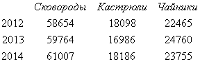
28 question.

Ellipse. Derivation of the Canonical Ellipse Equation. The form. Properties

An ellipse is the locus of points for which the sum of the distances from two fixed distances, called foci, is a given number 2a greater than the distance 2c between the foci.

https://pandia.ru/text/78/365/images/image195_4.gif" alt="(!LANG:image002" width="17" height="23 id=">.gif" alt="image043" width="81 height=44" height="44"> 0=!}

in Fig.2 r1=a+ex r2=a-ex

Ur-e tangent to ellipse

DIV_ADBLOCK417">

Canonical equation of a hyperbola

Form and St.

y=±b/a multiply by the root of (x2-a2)

The axis of symmetry of a hyperbola is its axes

Segment 2a - the real axis of the hyperbola

Eccentricity e=2c/2a=c/a

If b=a we get an isosceles hyperbola

An asymptote is a straight line if, with an unlimited removal of the point M1 along the curve, the distance from the point to the straight line tends to zero.

lim d=0 for x-> ∞

d=ba2/(x1+(x21-a2)1/2/c)

tangent of hyperbola

xx0/a2 - yy0/b2 = 1

parabola - the locus of points equidistant from a point called the focus and a given line called the directrix

Canonical parabola equation

properties

the axis of symmetry of the parabola passes through its focus and is perpendicular to the directrix

if you rotate the parabola, you get an elliptical paraboloid

all parabolas are similar

Question 30. Investigation of the equation of the general form of a curve of the second order.

Curve type def. with leading terms A1, B1, C1

A1x12+2Bx1y1+C1y12+2D1x1+2E1y1+F1=0

1. AC=0 ->curve of parabolic type

A=C=0 => 2Dx+2Ey+F=0

A≠0 C=0 => Ax2+2Dx+2Ey+F=0

If E=0 => Ax2+2Dx+F=0

then x1=x2 - merges into one

x1≠x2 - lines are parallel Oy

x1≠x2 and imaginary roots, has no geometric image

C≠0 A=0 =>C1y12+2D1x1+2E1y1+F1=0

Conclusion: a parabolic curve is either a parabola, or 2 parallel lines, or imaginary, or merge into one.

2.AC>0 -> elliptic type curve

Complementing the original equation to the full square, we transform it to the canonical one, then we get the cases

(x-x0)2/a2+(y-y0)2/b2=1 - ellipse

(x-x0)2/a2+(y-y0)2/b2=-1 - imaginary ellipse

(x-x0)2/a2-(y-y0)2/b2=0 - point with coordinate x0 y0

Conclusion: curve el. type is either an ellipse, or imaginary, or a point

3. AC<0 - кривая гиперболического типа

(x-x0)2/a2-(y-y0)2/b2=1 hyperbola, real axis is parallel

(x-x0)2/a2-(y-y0)2/b2=-1 hyperbola, real axis parallel to Oy

(x-x0)2/a2-(y-y0)2/b2=0 ur-e of two lines

Conclusion: a curve of hyperbolic type is either a hyperbola or two straight lines

Matrices in mathematics are one of the most important objects of applied importance. Often an excursion into the theory of matrices begins with the words: "A matrix is a rectangular table ...". We will start this excursion from a slightly different angle.

Phone books of any size and with any number of subscriber data are nothing but matrices. These matrices look like this:

It is clear that we all use such matrices almost every day. These matrices come in various numbers of rows (distinguished as a directory issued by the telephone company, which can contain thousands, hundreds of thousands, and even millions of lines, and a new notebook you just started, which has less than ten lines) and columns (a directory of officials of some some organization in which there may be columns such as position and office number and the same your notebook, where there may be no data other than the name, and, thus, it has only two columns - name and phone number).

All kinds of matrices can be added and multiplied, and other operations can be performed on them, but there is no need to add and multiply telephone directories, there is no benefit from this, and besides, you can move your mind.

But very many matrices can and should be added and multiplied and various urgent tasks can be solved in this way. Below are examples of such matrices.

Matrices in which the columns are the output of units of a particular type of product, and the rows are the years in which the output of this product is recorded:

You can add matrices of this kind, which take into account the production of similar products by various enterprises, in order to obtain summary data for the industry.

Or matrices, consisting, for example, of one column, in which the rows are the average cost of a particular type of product:

Matrices of the last two types can be multiplied, and the result is a row matrix containing the cost of all types of products by years.

Matrices, basic definitions

Rectangular table consisting of numbers arranged in m lines and n columns is called mn-matrix (or simply matrix ) and written like this:

(1)

In matrix (1) the numbers are called its elements (as in the determinant, the first index means the number of the row, the second - the column, at the intersection of which there is an element; i = 1, 2, ..., m; j = 1, 2, n).

The matrix is called rectangular , if .

If m = n, then the matrix is called square , and the number n is its in order .

The determinant of the square matrix A is called the determinant whose elements are the elements of the matrix A. It is denoted by the symbol | A|.

The square matrix is called non-special (or non-degenerate , non-singular ) if its determinant is not equal to zero, and special (or degenerate , singular ) if its determinant is zero.

The matrices are called equal if they have the same number of rows and columns and all matching elements are the same.

The matrix is called null if all its elements are equal to zero. The zero matrix will be denoted by the symbol 0 or .

For example,

row matrix (or lowercase ) is called 1 n-matrix, and column matrix (or columnar ) – m 1-matrix.

Matrix A" , which is obtained from the matrix A swapping rows and columns in it is called transposed with respect to the matrix A. Thus, for matrix (1), the transposed matrix is

Transition to matrix operation A" , transposed with respect to the matrix A, is called the transposition of the matrix A. For mn-matrix transposed is nm-matrix.

The matrix transposed with respect to the matrix is A, that is

(A")" = A .

Example 1 Find Matrix A" , transposed with respect to the matrix

and find out if the determinants of the original and transposed matrices are equal.

main diagonal A square matrix is an imaginary line connecting its elements, for which both indices are the same. These elements are called diagonal .

A square matrix in which all elements outside the main diagonal are equal to zero is called diagonal . Not all diagonal elements of a diagonal matrix are necessarily nonzero. Some of them may be equal to zero.

A square matrix in which the elements on the main diagonal are equal to the same non-zero number, and all others are equal to zero, is called scalar matrix .

identity matrix is called a diagonal matrix in which all diagonal elements are equal to one. For example, the identity matrix of the third order is the matrix

Example 2 Matrix data:

Solution. Let us calculate the determinants of these matrices. Using the rule of triangles, we find

Matrix determinant B calculate by the formula

We easily get that

Therefore, the matrices A and are non-singular (non-degenerate, non-singular), and the matrix B- special (degenerate, singular).

The determinant of an identity matrix of any order is obviously equal to one.

Solve the matrix problem yourself, and then see the solution

Example 3 Matrix data

Determine which of them are non-singular (non-degenerate, non-singular).

Application of matrices in mathematical and economic modeling

In the form of matrices, structured data about a particular object is simply and conveniently written. Matrix models are created not only to store this structured data, but also to solve various problems with this data using linear algebra.

Thus, the well-known matrix model of the economy is the input-output model introduced by the American economist of Russian origin Wassily Leontiev. This model is based on the assumption that the entire manufacturing sector of the economy is divided into n clean industries. Each of the industries produces only one type of product and different industries produce different products. Because of this division of labor between industries, there are inter-industry relations, the meaning of which is that part of the production of each industry is transferred to other industries as a production resource.

Production volume i-th industry (measured by a specific unit of measure) that was produced during the reporting period, denoted by and is called the total output i th industry. Issues are conveniently placed in n-component row of the matrix.

Number of product units i-th industry to be spent j-th industry for the production of a unit of its output, is denoted and called the coefficient of direct costs.