Dispersion measures. Calculation of group, intergroup and total variance (according to the rule of adding variances)

For grouped data residual dispersion- average of intragroup dispersions:

Where σ 2 j is the intra-group variance of the j -th group.

For ungrouped data residual dispersion is a measure of the approximation accuracy, i.e. approximation of the regression line to the original data: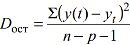
where y(t) is the forecast according to the trend equation; y t – initial series of dynamics; n is the number of points; p is the number of coefficients of the regression equation (the number of explanatory variables).
In this example it is called unbiased estimate of variance.

Example #1. The distribution of workers of three enterprises of one association by tariff categories is characterized by the following data:

Worker's wage category	Number of workers at the enterprise
	enterprise 1	enterprise 2	enterprise 3
1	50	20	40
2	100	80	60
3	150	150	200
4	350	300	400
5	200	150	250
6	150	100	150

Define:
1. dispersion for each enterprise (intragroup dispersion);
2. average of intragroup dispersions;
3. intergroup dispersion;
4. total variance.

Decision.
Before proceeding to solve the problem, it is necessary to find out which feature is effective and which is factorial. In the example under consideration, the effective feature is "Tariff category", and the factor feature is "Number (name) of the enterprise".
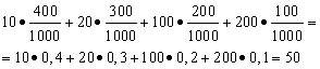
Then we have three groups (enterprises) for which it is necessary to calculate the group average and intragroup variances:

Company	group average,	within-group variance,
1	4	1,8

The average of the intragroup variances ( residual dispersion) calculated by the formula:

where you can calculate:
or:

then:
The total dispersion will be equal to: s 2 \u003d 1.6 + 0 \u003d 1.6.
The total variance can also be calculated using one of the following two formulas:

When solving practical problems, one often has to deal with a sign that takes only two alternative values. In this case, they are not talking about the weight of a particular value of a feature, but about its share in the aggregate. If the proportion of population units that have the trait under study is denoted by " R", and not possessing - through" q”, then the dispersion can be calculated by the formula:
s 2 = p×q

Example #2. Based on the data on the output of six workers of the brigade, determine the intergroup variance and evaluate the impact of the work shift on their labor productivity if the total variance is 12.2.

No. of the working brigade	Working output, pcs.
	in the first shift	in 2nd shift
1	18	13
2	19	14
3	22	15
4	20	17
5	24	16
6	23	15

Decision. Initial data

X	f1	f2	f 3	f4	f5	f6	Total
1	18	19	22	20	24	23	126
2	13	14	15	17	16	15	90
Total	31	33	37	37	40	38

Then we have 6 groups for which it is necessary to calculate the group mean and intragroup variances.
1. Find the average values ​​of each group.







2. Find the mean square of each group.







We summarize the results of the calculation in a table:

Group number	Group average	Intragroup variance
1	1.42	0.24
2	1.42	0.24
3	1.41	0.24
4	1.46	0.25
5	1.4	0.24
6	1.39	0.24

3. Intragroup variance characterizes the change (variation) of the studied (resulting) trait within the group under the influence of all factors, except for the factor underlying the grouping:
We calculate the average of the intragroup dispersions using the formula:


4. Intergroup variance characterizes the change (variation) of the studied (resulting) trait under the influence of a factor (factorial trait) underlying the grouping.
Intergroup dispersion is defined as:

where


Then

Total variance characterizes the change (variation) of the studied (resulting) trait under the influence of all factors (factorial traits) without exception. By the condition of the problem, it is equal to 12.2.
Empirical correlation relation measures how much of the total fluctuation of the resulting attribute is caused by the studied factor. This is the ratio of the factorial variance to the total variance:

We determine the empirical correlation relation:

Relationships between features can be weak or strong (close). Their criteria are evaluated on the Chaddock scale:
0.1 0.3 0.5 0.7 0.9 In our example, the relationship between feature Y factor X is weak
Determination coefficient.

Let's define the coefficient of determination:

Thus, 0.67% of the variation is due to differences between traits, and 99.37% is due to other factors.
Conclusion: in this case, the output of workers does not depend on work in a particular shift, i.e. the influence of the work shift on their labor productivity is not significant and is due to other factors.

Example #3. Based on the data on the average wage and the squared deviations from its value for two groups of workers, find the total variance by applying the variance addition rule:

Decision:
Average of within-group variances

Intergroup dispersion is defined as:


The total variance will be: 480 + 13824 = 14304

This page describes a standard example of finding the variance, you can also look at other tasks for finding it

Example 1. Determination of group, average of group, between-group and total variance

Example 2. Finding the variance and coefficient of variation in a grouping table

Example 3. Finding the variance in a discrete series

Example 4. We have the following data for a group of 20 correspondence students. It is necessary to build an interval series of the feature distribution, calculate the mean value of the feature and study its variance

Let's build an interval grouping. Let's determine the range of the interval by the formula:

where X max is the maximum value of the grouping feature;
X min is the minimum value of the grouping feature;
n is the number of intervals:

We accept n=5. The step is: h \u003d (192 - 159) / 5 \u003d 6.6

Let's make an interval grouping

For further calculations, we will build an auxiliary table:

X "i - the middle of the interval. (for example, the middle of the interval 159 - 165.6 \u003d 162.3)

The average growth of students is determined by the formula of the arithmetic weighted average:

We determine the dispersion by the formula:

The formula can be converted like this:

From this formula it follows that the variance is the difference between the mean of the squares of the options and the square and the mean.

Variance in variation series with equal intervals according to the method of moments can be calculated in the following way using the second property of the dispersion (dividing all options by the value of the interval). Definition of variance, calculated by the method of moments, according to the following formula is less time consuming:

where i is the value of the interval;
A - conditional zero, which is convenient to use the middle of the interval with the highest frequency;
m1 is the square of the moment of the first order;
m2 - moment of the second order

Feature variance (if in the statistical population the attribute changes in such a way that there are only two mutually exclusive options, then such variability is called alternative) can be calculated by the formula:

Substituting in this dispersion formula q = 1- p, we get:

Types of dispersion

Total variance measures the variation of a trait over the entire population as a whole under the influence of all the factors that cause this variation. It is equal to the mean square of the deviations of the individual values ​​of the feature x from the total mean value x and can be defined as simple variance or weighted variance.

Intragroup variance characterizes random variation, i.e. part of the variation, which is due to the influence of unaccounted for factors and does not depend on the sign-factor underlying the grouping. Such a variance is equal to the mean square of the deviations of the individual values ​​of a feature within the X group from the arithmetic mean of the group and can be calculated as a simple variance or as a weighted variance.

Thus, within-group variance measures variation of a trait within a group and is determined by the formula:

where xi - group average;
ni is the number of units in the group.

For example, intra-group variances that need to be determined in the task of studying the influence of workers' qualifications on the level of labor productivity in a shop show variations in output in each group caused by all possible factors (technical condition of equipment, availability of tools and materials, age of workers, labor intensity, etc. .), except for differences in the qualification category (within the group, all workers have the same qualification).

Mathematical expectation and variance are the most commonly used numerical characteristics of a random variable. They characterize the most important features of the distribution: its position and degree of dispersion. In many problems of practice, a complete, exhaustive description of a random variable - the law of distribution - either cannot be obtained at all, or is not needed at all. In these cases, they are limited to an approximate description of a random variable using numerical characteristics.

The mathematical expectation is often referred to simply as the average value of a random variable. Dispersion of a random variable is a characteristic of dispersion, dispersion of a random variable around its mathematical expectation.

Mathematical expectation of a discrete random variable

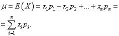
Let's approach the concept of mathematical expectation, first proceeding from the mechanical interpretation of the distribution of a discrete random variable. Let the unit mass be distributed between the points of the x-axis x1 , x 2 , ..., x n, and each material point has a mass corresponding to it from p1 , p 2 , ..., p n. It is required to choose one point on the x-axis, which characterizes the position of the entire system of material points, taking into account their masses. It is natural to take the center of mass of the system of material points as such a point. This is the weighted average of the random variable X, in which the abscissa of each point xi enters with a "weight" equal to the corresponding probability. The mean value of the random variable thus obtained X is called its mathematical expectation.

The mathematical expectation of a discrete random variable is the sum of the products of all its possible values ​​and the probabilities of these values:

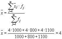
Example 1 Organized a win-win lottery. There are 1000 winnings, 400 of which are 10 rubles each. 300 - 20 rubles each 200 - 100 rubles each. and 100 - 200 rubles each. What is the average winnings for a person who buys one ticket?

Decision. We will find the average win if the total amount of winnings, which is equal to 10*400 + 20*300 + 100*200 + 200*100 = 50,000 rubles, is divided by 1000 (the total amount of winnings). Then we get 50000/1000 = 50 rubles. But the expression for calculating the average gain can also be represented in the following form:

On the other hand, under these conditions, the amount of winnings is a random variable that can take on the values ​​of 10, 20, 100 and 200 rubles. with probabilities equal to 0.4, respectively; 0.3; 0.2; 0.1. Therefore, the expected average payoff is equal to the sum of the products of the size of the payoffs and the probability of receiving them.

Example 2 The publisher decided to publish a new book. He is going to sell the book for 280 rubles, of which 200 will be given to him, 50 to the bookstore, and 30 to the author. The table gives information about the cost of publishing a book and the likelihood of selling a certain number of copies of the book.

Find the publisher's expected profit.

Decision. The random variable "profit" is equal to the difference between the income from the sale and the cost of the costs. For example, if 500 copies of a book are sold, then the income from the sale is 200 * 500 = 100,000, and the cost of publishing is 225,000 rubles. Thus, the publisher faces a loss of 125,000 rubles. The following table summarizes the expected values ​​of the random variable - profit:

Number	Profit xi	Probability pi	xi p i
500	-125000	0,20	-25000
1000	-50000	0,40	-20000
2000	100000	0,25	25000
3000	250000	0,10	25000
4000	400000	0,05	20000
Total:		1,00	25000

Thus, we obtain the mathematical expectation of the publisher's profit:

.

Example 3 Chance to hit with one shot p= 0.2. Determine the consumption of shells that provide the mathematical expectation of the number of hits equal to 5.

Decision. From the same expectation formula that we have used so far, we express x- consumption of shells:

.

Example 4 Determine the mathematical expectation of a random variable x number of hits with three shots, if the probability of hitting with each shot p = 0,4 .

Hint: find the probability of the values ​​of a random variable by Bernoulli formula .

Expectation Properties

Consider the properties of mathematical expectation.

Property 1. The mathematical expectation of a constant value is equal to this constant:

Property 2. The constant factor can be taken out of the expectation sign:

Property 3. The mathematical expectation of the sum (difference) of random variables is equal to the sum (difference) of their mathematical expectations:

Property 4. The mathematical expectation of the product of random variables is equal to the product of their mathematical expectations:

Property 5. If all values ​​of the random variable X decrease (increase) by the same number With, then its mathematical expectation will decrease (increase) by the same number:

When you can not be limited only to mathematical expectation

In most cases, only the mathematical expectation cannot adequately characterize a random variable.

Let random variables X and Y are given by the following distribution laws:

Meaning X	Probability
-0,1	0,1
-0,01	0,2
0	0,4
0,01	0,2
0,1	0,1

Meaning Y	Probability
-20	0,3
-10	0,1
0	0,2
10	0,1
20	0,3

The mathematical expectations of these quantities are the same - equal to zero:

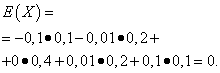
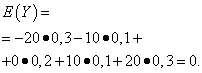
However, their distribution is different. Random value X can only take values ​​that are little different from the mathematical expectation, and the random variable Y can take values ​​that deviate significantly from the mathematical expectation. A similar example: the average wage does not make it possible to judge the proportion of high- and low-paid workers. In other words, by mathematical expectation one cannot judge what deviations from it, at least on average, are possible. To do this, you need to find the variance of a random variable.

Dispersion of a discrete random variable

dispersion discrete random variable X is called the mathematical expectation of the square of its deviation from the mathematical expectation:

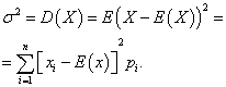
The standard deviation of a random variable X is the arithmetic value of the square root of its variance:

.

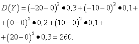
Example 5 Calculate variances and standard deviations of random variables X and Y, whose distribution laws are given in the tables above.

Decision. Mathematical expectations of random variables X and Y, as found above, are equal to zero. According to the dispersion formula for E(X)=E(y)=0 we get:

Then the standard deviations of random variables X and Y constitute

.

Thus, with the same mathematical expectations, the variance of the random variable X very small and random Y- significant. This is a consequence of the difference in their distribution.

Example 6 The investor has 4 alternative investment projects. The table summarizes the data on the expected profit in these projects with the corresponding probability.

Project 1	Project 2	Project 3	Project 4
500, P=1	1000, P=0,5	500, P=0,5	500, P=0,5
	0, P=0,5	1000, P=0,25	10500, P=0,25
		0, P=0,25	9500, P=0,25

Find for each alternative the mathematical expectation, variance and standard deviation.

Decision. Let us show how these quantities are calculated for the 3rd alternative:

The table summarizes the found values ​​for all alternatives.

All alternatives have the same mathematical expectation. This means that in the long run everyone has the same income. The standard deviation can be interpreted as a measure of risk - the larger it is, the greater the risk of the investment. An investor who doesn't want much risk will choose project 1 because it has the smallest standard deviation (0). If the investor prefers risk and high returns in a short period, then he will choose the project with the largest standard deviation - project 4.

Dispersion Properties

Let us present the properties of the dispersion.

Property 1. The dispersion of a constant value is zero:

Property 2. The constant factor can be taken out of the dispersion sign by squaring it:

.

Property 3. The variance of a random variable is equal to the mathematical expectation of the square of this value, from which the square of the mathematical expectation of the value itself is subtracted:

,

where .

Property 4. The variance of the sum (difference) of random variables is equal to the sum (difference) of their variances:

Example 7 It is known that a discrete random variable X takes only two values: −3 and 7. In addition, the mathematical expectation is known: E(X) = 4 . Find the variance of a discrete random variable.

Decision. Denote by p the probability with which a random variable takes on a value x1 = −3 . Then the probability of the value x2 = 7 will be 1 − p. Let's derive the equation for mathematical expectation:

E(X) = x 1 p + x 2 (1 − p) = −3p + 7(1 − p) = 4 ,

where we get the probabilities: p= 0.3 and 1 − p = 0,7 .

The law of distribution of a random variable:

X	−3	7
p	0,3	0,7

We calculate the variance of this random variable using the formula from property 3 of the variance:

D(X) = 2,7 + 34,3 − 16 = 21 .

Find the mathematical expectation of a random variable yourself, and then see the solution

Example 8 Discrete random variable X takes only two values. It takes the larger value of 3 with a probability of 0.4. In addition, the variance of the random variable is known D(X) = 6 . Find the mathematical expectation of a random variable.

Example 9 An urn contains 6 white and 4 black balls. 3 balls are taken from the urn. The number of white balls among the drawn balls is a discrete random variable X. Find the mathematical expectation and variance of this random variable.

Decision. Random value X can take the values ​​0, 1, 2, 3. The corresponding probabilities can be calculated from rule of multiplication of probabilities. The law of distribution of a random variable:

X	0	1	2	3
p	1/30	3/10	1/2	1/6

Hence the mathematical expectation of this random variable:

M(X) = 3/10 + 1 + 1/2 = 1,8 .

The variance of a given random variable is:

D(X) = 0,3 + 2 + 1,5 − 3,24 = 0,56 .

Mathematical expectation and dispersion of a continuous random variable

For a continuous random variable, the mechanical interpretation of the mathematical expectation will retain the same meaning: the center of mass for a unit mass distributed continuously on the x-axis with density f(x). In contrast to a discrete random variable, for which the function argument xi changes abruptly, for a continuous random variable, the argument changes continuously. But the mathematical expectation of a continuous random variable is also related to its mean value.

To find the mathematical expectation and variance of a continuous random variable, you need to find definite integrals . If a density function of a continuous random variable is given, then it enters directly into the integrand. If a probability distribution function is given, then by differentiating it, you need to find the density function.

The arithmetic average of all possible values ​​of a continuous random variable is called its mathematical expectation, denoted by or .

The dispersion of a random variable is a measure of the spread of the values ​​of this variable. Small variance means that the values ​​are clustered close to each other. A large variance indicates a strong scatter of values. The concept of the dispersion of a random variable is used in statistics. For example, if you compare the variance of the values ​​of two quantities (such as the results of observations of male and female patients), you can test the significance of some variable. Variance is also used when building statistical models, as small variance can be a sign that you are overfitting values.

Steps

Sample Variance Calculation

1. Record the sample values. In most cases, only samples of certain populations are available to statisticians. For example, as a rule, statisticians do not analyze the cost of maintaining the population of all cars in Russia - they analyze a random sample of several thousand cars. Such a sample will help determine the average cost per car, but most likely, the resulting value will be far from the real one.

   • For example, let's analyze the number of buns sold in a cafe in 6 days, taken in random order. The sample has the following form: 17, 15, 23, 7, 9, 13. This is a sample, not a population, because we do not have data on buns sold for each day the cafe is open.
   • If you are given a population and not a sample of values, skip to the next section.

2. Write down the formula for calculating the sample variance. Dispersion is a measure of the spread of values ​​of some quantity. The closer the dispersion value is to zero, the closer the values ​​are grouped together. When working with a sample of values, use the following formula to calculate the variance:

   • s 2 (\displaystyle s^(2)) = ∑[(x i (\displaystyle x_(i))-x̅) 2 (\displaystyle ^(2))] / (n - 1)
   • s 2 (\displaystyle s^(2)) is the dispersion. Dispersion is measured in square units.
   • x i (\displaystyle x_(i))- each value in the sample.
   • x i (\displaystyle x_(i)) you need to subtract x̅, square it, and then add the results.
   • x̅ – sample mean (sample mean).
   • n is the number of values ​​in the sample.

3. Calculate the sample mean. It is denoted as x̅. The sample mean is computed like a normal arithmetic mean: add up all the values ​​in the sample, and then divide the result by the number of values ​​in the sample.

   • In our example, add the values ​​in the sample: 15 + 17 + 23 + 7 + 9 + 13 = 84
     Now divide the result by the number of values ​​in the sample (in our example there are 6): 84 ÷ 6 = 14.
     Sample mean x̅ = 14.
   • The sample mean is the central value around which the values ​​in the sample are distributed. If the values ​​in the sample cluster around the sample mean, then the variance is small; otherwise, the dispersion is large.

4. Subtract the sample mean from each value in the sample. Now calculate the difference x i (\displaystyle x_(i))- x̅, where x i (\displaystyle x_(i))- each value in the sample. Each result indicates the degree of deviation of a particular value from the sample mean, that is, how far this value is from the sample mean.

   • In our example:
     x 1 (\displaystyle x_(1))- x̅ = 17 - 14 = 3
     x 2 (\displaystyle x_(2))- x̅ = 15 - 14 = 1
     x 3 (\displaystyle x_(3))- x̅ = 23 - 14 = 9
     x 4 (\displaystyle x_(4))- x̅ = 7 - 14 = -7
     x 5 (\displaystyle x_(5))- x̅ = 9 - 14 = -5
     x 6 (\displaystyle x_(6))- x̅ = 13 - 14 = -1
   • The correctness of the results obtained is easy to verify, since their sum must be equal to zero. This is related to the determination of the average value, since negative values ​​(distances from the average value to smaller values) are completely offset by positive values ​​(distances from the average value to larger values).

5. As noted above, the sum of the differences x i (\displaystyle x_(i))- x̅ must be equal to zero. This means that the mean variance is always zero, which does not give any idea of ​​the spread of the values ​​of some quantity. To solve this problem, square each difference x i (\displaystyle x_(i))- x̅. This will result in you only getting positive numbers which, when added together, will never add up to 0.

   • In our example:
     (x 1 (\displaystyle x_(1))-x̅) 2 = 3 2 = 9 (\displaystyle ^(2)=3^(2)=9)
     (x 2 (\displaystyle (x_(2))-x̅) 2 = 1 2 = 1 (\displaystyle ^(2)=1^(2)=1)
     9 2 = 81
     (-7) 2 = 49
     (-5) 2 = 25
     (-1) 2 = 1
   • You have found the square of the difference - x̅) 2 (\displaystyle ^(2)) for each value in the sample.

6. Calculate the sum of squared differences. That is, find the part of the formula that is written like this: ∑[( x i (\displaystyle x_(i))-x̅) 2 (\displaystyle ^(2))]. Here the sign Σ means the sum of squared differences for each value x i (\displaystyle x_(i)) in the sample. You have already found the squared differences (x i (\displaystyle (x_(i))-x̅) 2 (\displaystyle ^(2)) for each value x i (\displaystyle x_(i)) in the sample; now just add these squares.

   • In our example: 9 + 1 + 81 + 49 + 25 + 1 = 166 .

7. Divide the result by n - 1, where n is the number of values ​​in the sample. Some time ago, to calculate the sample variance, statisticians simply divided the result by n; in this case, you will get the mean of the squared variance, which is ideal for describing the variance of a given sample. But remember that any sample is only a small part of the general population of values. If you take a different sample and do the same calculations, you'll get a different result. As it turns out, dividing by n - 1 (rather than just n) gives a better estimate of the population variance, which is what you're after. Dividing by n - 1 has become commonplace, so it is included in the formula for calculating the sample variance.

   • In our example, the sample includes 6 values, that is, n = 6.
     Sample variance = s 2 = 166 6 − 1 = (\displaystyle s^(2)=(\frac (166)(6-1))=) 33,2

8. The difference between the variance and the standard deviation. Note that the formula contains an exponent, so the variance is measured in square units of the analyzed value. Sometimes such a value is quite difficult to operate; in such cases, the standard deviation is used, which is equal to the square root of the variance. That is why the sample variance is denoted as s 2 (\displaystyle s^(2)), and the sample standard deviation as s (\displaystyle s).

   • In our example, the sample standard deviation is: s = √33.2 = 5.76.

   Population variance calculation

   1. Analyze some set of values. The set includes all values ​​of the quantity under consideration. For example, if you are studying the age of residents of the Leningrad region, then the population includes the age of all residents of this region. In the case of working with an aggregate, it is recommended to create a table and enter the values ​​of the aggregate into it. Consider the following example:

      • There are 6 aquariums in a certain room. Each aquarium contains the following number of fish:
        x 1 = 5 (\displaystyle x_(1)=5)
        x 2 = 5 (\displaystyle x_(2)=5)
        x 3 = 8 (\displaystyle x_(3)=8)
        x 4 = 12 (\displaystyle x_(4)=12)
        x 5 = 15 (\displaystyle x_(5)=15)
        x 6 = 18 (\displaystyle x_(6)=18)

   2. Write down the formula for calculating the population variance. Since the population includes all values ​​of a certain quantity, the following formula allows you to get the exact value of the variance of the population. To distinguish population variance from sample variance (which is only an estimate), statisticians use various variables:

      • σ 2 (\displaystyle ^(2)) = (∑(x i (\displaystyle x_(i)) - μ) 2 (\displaystyle ^(2))) / n
      • σ 2 (\displaystyle ^(2))- population variance (read as "sigma squared"). Dispersion is measured in square units.
      • x i (\displaystyle x_(i))- each value in the aggregate.
      • Σ is the sign of the sum. That is, for each value x i (\displaystyle x_(i)) subtract μ, square it, and then add the results.
      • μ is the population mean.
      • n is the number of values ​​in the general population.

   3. Calculate the population mean. When working with the general population, its average value is denoted as μ (mu). The population mean is calculated as the usual arithmetic mean: add up all the values ​​in the population, and then divide the result by the number of values ​​in the population.

      • Keep in mind that averages are not always calculated as the arithmetic mean.
      • In our example, the population mean: μ = 5 + 5 + 8 + 12 + 15 + 18 6 (\displaystyle (\frac (5+5+8+12+15+18)(6))) = 10,5

   4. Subtract the population mean from each value in the population. The closer the difference value is to zero, the closer the particular value is to the population mean. Find the difference between each value in the population and its mean, and you'll get a first look at the distribution of the values.

      • In our example:
        x 1 (\displaystyle x_(1))- μ = 5 - 10.5 = -5.5
        x 2 (\displaystyle x_(2))- μ = 5 - 10.5 = -5.5
        x 3 (\displaystyle x_(3))- μ = 8 - 10.5 = -2.5
        x 4 (\displaystyle x_(4))- μ = 12 - 10.5 = 1.5
        x 5 (\displaystyle x_(5))- μ = 15 - 10.5 = 4.5
        x 6 (\displaystyle x_(6))- μ = 18 - 10.5 = 7.5

   5. Square each result you get. The difference values ​​will be both positive and negative; if you put these values ​​on a number line, then they will lie to the right and left of the population mean. This is not good for calculating variance, as positive and negative numbers cancel each other out. Therefore, square each difference to get exclusively positive numbers.

      • In our example:
        (x i (\displaystyle x_(i)) - μ) 2 (\displaystyle ^(2)) for each population value (from i = 1 to i = 6):
        (-5,5)2 (\displaystyle ^(2)) = 30,25
        (-5,5)2 (\displaystyle ^(2)), where x n (\displaystyle x_(n)) is the last value in the population.
      • To calculate the average value of the results obtained, you need to find their sum and divide it by n: (( x 1 (\displaystyle x_(1)) - μ) 2 (\displaystyle ^(2)) + (x 2 (\displaystyle x_(2)) - μ) 2 (\displaystyle ^(2)) + ... + (x n (\displaystyle x_(n)) - μ) 2 (\displaystyle ^(2))) / n
      • Now let's write the above explanation using variables: (∑( x i (\displaystyle x_(i)) - μ) 2 (\displaystyle ^(2))) / n and obtain a formula for calculating the population variance.

Dispersion in statistics is found as individual values ​​of the feature in the square of . Depending on the initial data, it is determined by the simple and weighted variance formulas:

1. (for ungrouped data) is calculated by the formula:

2. Weighted variance (for a variation series):

where n is the frequency (repeatability factor X)

An example of finding the variance

This page describes a standard example of finding the variance, you can also look at other tasks for finding it

Example 1. We have the following data for a group of 20 correspondence students. It is necessary to build an interval series of the feature distribution, calculate the mean value of the feature and study its variance

Let's build an interval grouping. Let's determine the range of the interval by the formula:

where X max is the maximum value of the grouping feature;
X min is the minimum value of the grouping feature;
n is the number of intervals:

We accept n=5. The step is: h \u003d (192 - 159) / 5 \u003d 6.6

Let's make an interval grouping

For further calculations, we will build an auxiliary table:

X'i is the middle of the interval. (for example, the middle of the interval 159 - 165.6 = 162.3)

The average growth of students is determined by the formula of the arithmetic weighted average:

We determine the dispersion by the formula:

The variance formula can be converted as follows:

From this formula it follows that the variance is the difference between the mean of the squares of the options and the square and the mean.

Variance in variation series with equal intervals according to the method of moments can be calculated in the following way using the second property of the dispersion (dividing all options by the value of the interval). Definition of variance, calculated by the method of moments, according to the following formula is less time consuming:

where i is the value of the interval;
A - conditional zero, which is convenient to use the middle of the interval with the highest frequency;
m1 is the square of the moment of the first order;
m2 - moment of the second order

(if in the statistical population the attribute changes in such a way that there are only two mutually exclusive options, then such variability is called alternative) can be calculated by the formula:

Substituting in this dispersion formula q = 1- p, we get:

Types of dispersion

Total variance measures the variation of a trait over the entire population as a whole under the influence of all the factors that cause this variation. It is equal to the mean square of the deviations of the individual values ​​of the feature x from the total mean value x and can be defined as simple variance or weighted variance.

characterizes random variation, i.e. part of the variation, which is due to the influence of unaccounted for factors and does not depend on the sign-factor underlying the grouping. Such a variance is equal to the mean square of the deviations of the individual values ​​of a feature within the X group from the arithmetic mean of the group and can be calculated as a simple variance or as a weighted variance.

Thus, within-group variance measures variation of a trait within a group and is determined by the formula:

where xi - group average;
ni is the number of units in the group.

For example, intra-group variances that need to be determined in the task of studying the influence of workers' qualifications on the level of labor productivity in a shop show variations in output in each group caused by all possible factors (technical condition of equipment, availability of tools and materials, age of workers, labor intensity, etc. .), except for differences in the qualification category (within the group, all workers have the same qualification).

The average of the within-group variances reflects the random, i.e., that part of the variation that occurred under the influence of all other factors, with the exception of the grouping factor. It is calculated by the formula:

It characterizes the systematic variation of the resulting trait, which is due to the influence of the trait-factor underlying the grouping. It is equal to the mean square of the deviations of the group means from the overall mean. Intergroup variance is calculated by the formula:

Variance addition rule in statistics

According to variance addition rule the total variance is equal to the sum of the average of the intragroup and intergroup variances:

The meaning of this rule is that the total variance that occurs under the influence of all factors is equal to the sum of the variances that arise under the influence of all other factors and the variance that arises due to the grouping factor.

Using the formula for adding variances, it is possible to determine the third unknown from two known variances, and also to judge the strength of the influence of the grouping attribute.

Dispersion Properties

1. If all the values ​​of the attribute are reduced (increased) by the same constant value, then the variance will not change from this.
2. If all the values ​​of the attribute are reduced (increased) by the same number of times n, then the variance will accordingly decrease (increase) by n^2 times.