How to calculate the arithmetic mean in excel. Calculation of the arithmetic mean in Excel

17.02.2017

Excel is a spreadsheet. It can be used to create a variety of reports. In this program, it is very convenient to perform various calculations. Many do not use even half of Excel's capabilities.

You may need to find the average value of numbers at school, as well as during work. The classic way to determine the arithmetic mean without using programs is to add all the numbers, and then divide the resulting sum by the number of terms. If the numbers are large enough, or if the operation needs to be performed many times for reporting purposes, the calculations can take a long time. This is an irrational waste of time and effort, it is much better to use the capabilities of Excel.

Finding the arithmetic mean

Many data are already initially recorded in Excel, but if this does not happen, it is necessary to transfer the data to a table. Each number for the calculation must be in a separate cell.

Method 1: Calculate the average value through the "Function Wizard"

In this method, you need to write a formula for calculating the arithmetic mean and apply it to the specified cells.

The main inconvenience of this method is that you have to manually enter cells for each term. If there are a lot of numbers, this is not very convenient.

Method 2: Automatic calculation of the result in selected cells

In this method, the calculation of the arithmetic mean is carried out in just a couple of mouse clicks. Very handy for any number of numbers.

The disadvantage of this method is the calculation of the average value only for numbers located nearby. If the necessary terms are scattered, then they cannot be selected for calculation. It is not even possible to select two columns, in which case the results will be presented separately for each of them.

Method 3: Using the formula bar

Another way to go to the function window:

The fastest way, in which you do not need to search for a long time in the menu, you need items.

Method 4: Manual Entry

It is not necessary to use the tools in the Excel menu to calculate the average value, you can manually write the necessary function.

A quick and convenient way for those who prefer to create formulas with their own hands, rather than looking for ready-made programs in the menu.

Thanks to these features, it is very easy to calculate the average value of any numbers, regardless of their number, and you can also compile statistics without manually calculating them. With the help of the tools of the Excel program, any calculations are much easier to make than in the mind or using a calculator.

In the process of various calculations and work with data, it is often necessary to calculate their average value. It is calculated by adding the numbers and dividing the total by their number. Let's find out how to calculate the average of a set of numbers using Microsoft Excel in various ways.

The easiest and most well-known way to find the arithmetic mean of a set of numbers is to use the special button on the Microsoft Excel ribbon. We select a range of numbers located in a column or line of a document. Being in the "Home" tab, click on the "Autosum" button, which is located on the ribbon in the "Editing" tool block. Select "Average" from the drop-down list.

After that, using the "AVERAGE" function, the calculation is made. In the cell under the selected column, or to the right of the selected row, the arithmetic mean of the given set of numbers is displayed.

This method is good for simplicity and convenience. But, it also has significant drawbacks. Using this method, you can calculate the average value of only those numbers that are arranged in a row in one column, or in one row. But, with an array of cells, or with scattered cells on a sheet, you cannot work using this method.

For example, if you select two columns and calculate the arithmetic mean using the above method, then the answer will be given for each column separately, and not for the entire array of cells.

Calculation with the Function Wizard

For cases where you need to calculate the arithmetic mean of an array of cells, or scattered cells, you can use the Function Wizard. It still uses the same AVERAGE function we know from the first calculation method, but it does it in a slightly different way.

We click on the cell where we want the result of calculating the average value to be displayed. Click on the "Insert Function" button, which is located to the left of the formula bar. Or, we type the combination Shift + F3 on the keyboard.

The Function Wizard starts. In the list of functions presented, we are looking for "AVERAGE". Select it and click on the "OK" button.

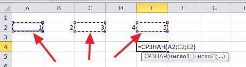
The arguments window for this function opens. Function arguments are entered into the "Number" fields. These can be both ordinary numbers and cell addresses where these numbers are located. If it is inconvenient for you to enter cell addresses manually, then you should click on the button located to the right of the data entry field.

After that, the function arguments window will collapse, and you can select the group of cells on the sheet that you take for calculation. Then, again click on the button to the left of the data entry field to return to the function arguments window.

If you want to calculate the arithmetic mean between the numbers in disparate groups of cells, then do the same steps as mentioned above in the "Number 2" field. And so on until all the desired groups of cells are selected.

After that, click on the "OK" button.

The result of calculating the arithmetic mean will be highlighted in the cell that you selected before starting the Function Wizard.

Formula bar

There is a third way to run the "AVERAGE" function. To do this, go to the Formulas tab. Select the cell in which the result will be displayed. After that, in the group of tools "Library of functions" on the ribbon, click on the button "Other functions". A list appears in which you need to sequentially go through the items "Statistical" and "AVERAGE".

Then, exactly the same function arguments window is launched, as when using the Function Wizard, the work in which we described in detail above.

The next steps are exactly the same.

Manual function entry

But, do not forget that you can always enter the "AVERAGE" function manually if you wish. It will have the following pattern: "=AVERAGE(cell_range_address(number); cell_range_address(number)).

Of course, this method is not as convenient as the previous ones, and requires certain formulas to be kept in the user's head, but it is more flexible.

Calculation of the average value by condition

In addition to the usual calculation of the average value, it is possible to calculate the average value by condition. In this case, only those numbers from the selected range that meet a certain condition will be taken into account. For example, if these numbers are greater or less than a specific value.

For these purposes, the AVERAGEIF function is used. Like the AVERAGE function, you can run it through the Function Wizard, from the formula bar, or by manually entering it into a cell. After the function arguments window has opened, you need to enter its parameters. In the "Range" field, enter the range of cells whose values ​​will be used to determine the arithmetic mean. We do this in the same way as with the AVERAGE function.

And here, in the "Condition" field, we must specify a specific value, numbers greater or less than which will be involved in the calculation. This can be done using comparison signs. For example, we took the expression ">=15000". That is, only cells in the range containing numbers greater than or equal to 15000 will be taken for calculation. If necessary, instead of a specific number, you can specify the address of the cell in which the corresponding number is located.

The field "Averaging range" is optional. Entering data into it is required only when using cells with text content.

When all the data is entered, click on the "OK" button.

After that, the result of the calculation of the arithmetic average for the selected range is displayed in the pre-selected cell, with the exception of cells whose data do not meet the conditions.

As you can see, in Microsoft Excel there are a number of tools with which you can calculate the average value of a selected series of numbers. Moreover, there is a function that automatically selects numbers from a range that do not meet a user-defined criteria. This makes calculations in Microsoft Excel even more user-friendly.

When working with tables in Excel, it often becomes necessary to calculate the sum or average. We have already talked about how to calculate the amount.

How to calculate the average of a column, row, or individual cells

The easiest way is to calculate the average value of a column or row. To do this, you must first select a series of numbers that are placed in a column or in a row. After the numbers are selected, you need to use the "Auto sum" button, which is located on the "Home" tab. Click on the arrow to the right of this button and select "Average" from the menu that appears.

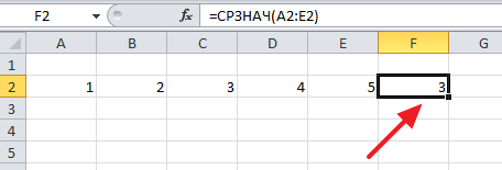
As a result, their average value will appear next to the numbers. If you look at the line for formulas, it becomes clear that Excel uses the AVERAGE function to get the average value. You can use this feature anywhere and without the "Auto Sum" button.

If you need the middle value to appear in some other cell, then you can transfer the result by simply cutting it (CTRL-X) and then pasting (CTRL-V). Or you can first select the cell where the result should be, and then click on the "Auto Sum - Average" button and select a series of numbers.

If you need to calculate the average value of some individual or specific cells, then this can also be done using the "Auto Sum - Average" button. In this case, you must first select the cell in which the result will be located, then click "Auto Sum - Average" and select the cells for which you want to calculate the average value. To select individual cells, hold down the CTRL key on your keyboard.

In addition, you can enter a formula to calculate the average value of certain cells manually. To do this, you need to put the cursor where the result should be, and then enter the formula in the format: = AVERAGE (D3; D5; D7). Where instead of D3, D5 and D7 you need to specify the addresses of the data cells you need.

It should be noted that when entering the formula manually, cell addresses are entered separated by commas, and a comma is not placed after the last cell. After entering the entire formula, you need to press the Enter key to save the result.

How to quickly calculate and view the average in Excel

In addition to all of the above, Excel has the ability to quickly calculate and view the average value of any data. To do this, you just need to select the desired cells and look in the lower right corner of the program window.

There will be indicated the average value of the selected cells, as well as their number and sum.

How to calculate the average of numbers in Excel

You can find the arithmetic mean of numbers in Excel using the function.

Syntax AVERAGE

=AVERAGE(number1,[number2],…) - Russian version

Arguments AVERAGE

• number1- the first number or range of numbers, for calculating the arithmetic mean;
• number2(Optional) – second number or range of numbers to calculate the arithmetic mean. The maximum number of function arguments is 255.

To calculate, do the following steps:

• Select any cell;
• Write a formula in it =AVERAGE(
• Select the range of cells for which you want to make a calculation;
• Press the "Enter" key on the keyboard

The function will calculate the average value in the specified range among those cells that contain numbers.

How to find the average value given text

If there are empty lines or text in the data range, then the function treats them as "zero". If there are logical expressions FALSE or TRUE among the data, then the function perceives FALSE as “zero”, and TRUE as “1”.

How to find the arithmetic mean by condition

The function is used to calculate the average by a condition or criterion. For example, let's say we have product sales data:

Our task is to calculate the average sales of pens. To do this, we will take the following steps:

• In a cell A13 write the name of the product “Pens”;
• In a cell B13 let's enter the formula:

=AVERAGEIF(A2:A10,A13,B2:B10)

Cell range “ A2:A10” points to the list of products in which we will search for the word “Pens”. Argument A13 this is a link to a cell with text that we will search for among the entire list of products. Cell range “ B2:B10” is a range with product sales data, among which the function will find “Pens” and calculate the average value.

Arithmetic mean in excel. Excel spreadsheets are the best suited for all kinds of calculations. Having studied Excel, you will be able to solve problems in chemistry, physics, mathematics, geometry, biology, statistics, economics and many others. We do not even think about what a powerful tool is on our computers, which means we do not use it to its full potential. Many parents think that a computer is just an expensive toy. But in vain! Of course, in order for the child to really study on it, you yourself need to learn how to work on it, and then teach the child. Well, this is another topic, but today I want to talk with you about how to find the arithmetic mean in Excel.

How to find the arithmetic mean in Excel

We have already talked about fast in Excel, and today we will talk about the arithmetic mean.

Select a cell C12 and with the help Function Wizards write in it the formula for calculating the arithmetic mean. To do this, on the Standard toolbar, click on the button - Inserting a Function −fx (in the picture above, the red arrow is on top). A dialog box will open Function Master .

• Select in the field Categories — Statistical ;
• In field Select function: AVERAGE ;
• Click the button OK .

The following window will open Arguments and Functions .

In field Number1 you will see the entry S2:S11- the program itself determined the range of cells for which it is necessary find the arithmetic mean.

Click the button OK and in the cell C12 the arithmetic mean of the scores will appear.

It turns out that calculating the arithmetic mean in excel is not at all difficult. And I was always afraid of any formulas. Eh, not at that time we studied.