Checkmate expectation x y. Mathematical expectation, definition, mathematical expectation of discrete and continuous random variables, selective, conditional expectation, calculation, properties, tasks, estimation of expectation, variance, distribution function, formulas, examples

The mathematical expectation is, the definition

Mat waiting is one of the most important concepts in mathematical statistics and probability theory, characterizing the distribution of values ​​or probabilities random variable. Usually expressed as a weighted average of all possible parameters of a random variable. It is widely used in technical analysis, the study of number series, the study of continuous and long-term processes. It is important in assessing risks, predicting price indicators when trading in financial markets, and is used in the development of strategies and methods of game tactics in gambling theory.

Checkmate waiting- This mean value of a random variable, distribution probabilities random variable is considered in probability theory.

Mat waiting is measure of the mean value of a random variable in probability theory. Math expectation of a random variable x denoted M(x).

Mathematical expectation (Population mean) is

Mat waiting is

Mat waiting is in probability theory, the weighted average of all possible values ​​that this random variable can take.

Mat waiting is the sum of the products of all possible values ​​of a random variable by the probabilities of these values.

Mathematical expectation (Population mean) is

Mat waiting is the average benefit from a particular decision, provided that such a decision can be considered in the framework of the theory of large numbers and a long distance.

Mat waiting is in the theory of gambling, the amount of winnings that a speculator can earn or lose, on average, for each bet. In the language of gambling speculators this is sometimes called the "advantage speculator” (if it is positive for the speculator) or “house edge” (if it is negative for the speculator).

Mathematical expectation (Population mean) is

Mat waiting is profit per win multiplied by the average profit, minus the loss multiplied by the average loss.

Mathematical expectation of a random variable in mathematical theory

One of the important numerical characteristics of a random variable is the expectation. Let us introduce the concept of a system of random variables. Consider a set of random variables that are the results of the same random experiment. If is one of the possible values ​​of the system, then the event corresponds to a certain probability that satisfies Kolmogorov's axioms. A function defined for any possible values ​​of random variables is called a joint distribution law. This function allows you to calculate the probabilities of any events from. In particular, joint law distribution of random variables and, which take values ​​from the set and, is given by probabilities.

The term "mat. expectation” was introduced by Pierre Simon Marquis de Laplace (1795) and originated from the concept of “expected value of the payoff”, which first appeared in the 17th century in the theory of gambling in the works of Blaise Pascal and Christian Huygens. However, the first complete theoretical understanding and evaluation of this concept was given by Pafnuty Lvovich Chebyshev (mid-19th century).

Law distributions of random numerical variables (distribution function and distribution series or probability density) completely describe the behavior of a random variable. But in a number of problems it is enough to know some numerical characteristics of the quantity under study (for example, its average value and possible deviation from it) in order to answer the question posed. The main numerical characteristics of random variables are expectation, variance, mode and median.

Math expectation of a discrete random variable is the sum of the products of its possible values ​​and their corresponding probabilities. Sometimes mat. the expectation is called the weighted average, since it is approximately equal to the arithmetic mean of the observed values ​​of the random variable over a large number of experiments. From the definition of the expectation mat, it follows that its value is not less than the smallest possible value of a random variable and not more than the largest. Math expectation of a random variable is a non-random (constant) variable.

Math expectation has a simple physical meaning: if a unit mass is placed on a straight line, placing some mass at some points (for a discrete distribution), or “smearing” it with a certain density (for an absolutely continuous distribution), then the point corresponding to the mat expectation will be the coordinate "center of gravity" straight.

The average value of a random variable is a certain number, which is, as it were, its “representative” and replaces it in rough approximate calculations. When we say: “the average lamp operation time is 100 hours” or “the average point of impact is shifted relative to the target by 2 m to the right”, we indicate by this a certain numerical characteristic of a random variable that describes its location on the numerical axis, i.e. position description.

Of the characteristics of the situation in the theory of probability, the most important role is played by the expectation of a random variable, which is sometimes called simply the average value of a random variable.

Consider a random variable X, which has possible values x1, x2, …, xn with probabilities p1, p2, …, pn. We need to characterize by some number the position of the values ​​of the random variable on the x-axis with taking into account that these values ​​have different probabilities. For this purpose, it is natural to use the so-called "weighted average" of the values xi, and each value xi during averaging should be taken into account with a “weight” proportional to the probability of this value. Thus, we will calculate the mean of the random variable X, which we will denote M|X|:

This weighted average is called the mat expectation of the random variable. Thus, we introduced in consideration one of the most important concepts of probability theory - the concept of mat. expectations. Mat. The expectation of a random variable is the sum of the products of all possible values ​​of a random variable and the probabilities of these values.

Mat. expectation of a random variable X due to a peculiar dependence with the arithmetic mean of the observed values ​​of a random variable with a large number of experiments. This dependence is of the same type as the dependence between frequency and probability, namely: with a large number of experiments, the arithmetic mean of the observed values ​​of a random variable approaches (converges in probability) to its mat. waiting. From the presence of a relationship between frequency and probability, one can deduce as a consequence the existence of a similar relationship between the arithmetic mean and mathematical expectation. Indeed, consider a random variable X, characterized by a series of distributions:

Let it be produced N independent experiments, in each of which the value X takes on a certain value. Suppose the value x1 appeared m1 times, value x2 appeared m2 times, general meaning xi appeared mi times. Let us calculate the arithmetic mean of the observed values ​​of X, which, in contrast to the expectation mats M|X| we will denote M*|X|:

With an increase in the number of experiments N frequencies pi will approach (converge in probability) the corresponding probabilities. Therefore, the arithmetic mean of the observed values ​​of the random variable M|X| with an increase in the number of experiments, it will approach (converge in probability) to its expectation. The relation formulated above between the arithmetic mean and the mat. expectation is the content of one of the forms of the law of large numbers.

We already know that all forms of the law of large numbers state the fact that certain averages are stable over a large number of experiments. Here we are talking about the stability of the arithmetic mean from a series of observations of the same value. With a small number of experiments, the arithmetic mean of their results is random; with a sufficient increase in the number of experiments, it becomes "almost not random" and, stabilizing, approaches a constant value - mat. waiting.

The property of stability of averages for a large number of experiments is easy to verify experimentally. For example, weighing any body in the laboratory on accurate scales, as a result of weighing we get a new value each time; to reduce the error of observation, we weigh the body several times and use the arithmetic mean of the obtained values. It is easy to see that with a further increase in the number of experiments (weighings), the arithmetic mean reacts to this increase less and less, and with a sufficiently large number of experiments it practically ceases to change.

It should be noted that the most important characteristic of the position of a random variable is mat. expectation - does not exist for all random variables. It is possible to make examples of such random variables for which mat. there is no expectation, since the corresponding sum or integral diverges. However, for practice, such cases are not of significant interest. Usually, the random variables we deal with have a limited range of possible values ​​and, of course, have a mat expectation.

In addition to the most important of the characteristics of the position of a random variable - the expectation value - other characteristics of the position are sometimes used in practice, in particular, the mode and median of the random variable.

The mode of a random variable is its most probable value. The term "most likely value", strictly speaking, applies only to discontinuous quantities; for a continuous quantity, the mode is the value at which the probability density is maximum. The figures show the mode for discontinuous and continuous random variables, respectively.

If the distribution polygon (distribution curve) has more than one maximum, the distribution is said to be "polymodal".

Sometimes there are distributions that have in the middle not a maximum, but a minimum. Such distributions are called "antimodal".

In the general case, the mode and expectation of a random variable do not coincide. In the special case when the distribution is symmetric and modal (i.e. has a mode) and there is a mat. expectation, then it coincides with the mode and the center of symmetry of the distribution.

Another characteristic of the position is often used - the so-called median of a random variable. This characteristic is usually used only for continuous random variables, although it can be formally defined for a discontinuous variable as well. Geometrically, the median is the abscissa of the point at which the area bounded by the distribution curve is bisected.

In the case of a symmetric modal distribution, the median coincides with the mat. expectation and fashion.

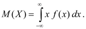
Math expectation is an average value, random variable - a numerical characteristic of the probability distribution of a random variable. In the most general way, the mat expectation of a random variable X(w) is defined as the Lebesgue integral with respect to the probability measure R in the original probability space:

Mat. expectation can also be calculated as the Lebesgue integral of X by probability distribution px quantities X:

In a natural way, one can define the concept of a random variable with infinite expectation. A typical example is the repatriation times in some random walks.

With the help of mat. expectations are defined by many numerical and functional characteristics of the distribution (as the mathematical expectation of the corresponding functions of a random variable), for example, generating function, characteristic function, moments of any order, in particular variance, covariance.

Mathematical expectation (Population mean) is

Math expectation is a characteristic of the location of the values ​​of a random variable (the average value of its distribution). In this capacity, the mathematical expectation serves as some "typical" distribution parameter and its role is similar to the role of the static moment - the coordinate of the center of gravity of the mass distribution - in mechanics. From other characteristics of the location, with the help of which the distribution is described in general terms - medians, modes, expectation differs in the greater value that it and the corresponding scattering characteristic - variance - have in the limit theorems of probability theory. With the greatest completeness, the meaning of expectation mats is revealed by the law of large numbers (Chebyshev's inequality) and the strengthened law of large numbers.

Mathematical expectation (Population mean) is

Mathematical expectation of a discrete random variable

Let there be some random variable that can take one of several numerical values ​​(for example, the number of points in a die roll can be 1, 2, 3, 4, 5, or 6). Often in practice, for such a value, the question arises: what value does it take "on average" with a large number of tests? What will be our average return (or loss) from each of the risky transactions?

Let's say there is some kind of lottery. We want to understand whether it is profitable or not to participate in it (or even participate repeatedly, regularly). Let's say that every fourth ticket wins, the prize will be 300 rubles, and any ticket - 100 rubles. With an infinite number of participations, this is what happens. In three-quarters of the cases, we will lose, every three losses will cost 300 rubles. In every fourth case, we will win 200 rubles. (prize minus cost), that is, for four participations, we lose an average of 100 rubles, for one - an average of 25 rubles. In total, the average rate of our ruin will be 25 rubles per ticket.

We throw a dice. If it's not cheating (without shifting the center of gravity, etc.), then how many points will we have on average at a time? Since each option is equally likely, we take the stupid arithmetic mean and get 3.5. Since this is AVERAGE, there is no need to be indignant that no particular throw will give 3.5 points - well, this cube does not have a face with such a number!

Now let's summarize our examples:

Let's take a look at the picture just above. On the left is a table of the distribution of a random variable. The value of X can take one of n possible values ​​(given in the top row). There can be no other values. Under each possible value, its probability is signed below. On the right is a formula, where M(X) is called mat. waiting. The meaning of this value is that with a large number of trials (with a large sample), the average value will tend to this very expectation.

Let's go back to the same playing cube. Mat. the expectation of the number of points when throwing is 3.5 (calculate yourself using the formula if you don’t believe it). Let's say you threw it a couple of times. 4 and 6 fell out. On average, it turned out 5, that is, far from 3.5. They threw it again, 3 fell out, that is, on average (4 + 6 + 3) / 3 = 4.3333 ... Somehow far from the mat. expectations. Now do a crazy experiment - roll the cube 1000 times! And if the average is not exactly 3.5, then it will be close to that.

Let's count mat. waiting for the above described lottery. The table will look like this:

Then the expectation checkmate will be, as we have established above.:

Another thing is that it is also "on the fingers", without a formula, it would be difficult if there were more options. Well, let's say there were 75% losing tickets, 20% winning tickets, and 5% winning tickets.

Now some properties of expectation mat.

Mat. the wait is linear. It's easy to prove it:

The constant multiplier is allowed to be taken out of the checkmate sign. expectations, that is:

This is a special case of the linearity property of expectation mats.

Another consequence of the linearity of mat. expectations:

that is mat. the expectation of the sum of random variables is equal to the sum of mathematical expectations of random variables.

Let X, Y be independent random variables, then:

This is also easy to prove) XY itself is a random variable, while if the initial values ​​could take n and m values, respectively, then XY can take nm values. each of the values ​​is calculated based on the fact that the probabilities of independent events are multiplied. As a result, we get this:

Mathematical expectation of a continuous random variable

Continuous random variables have such a characteristic as the distribution density (probability density). It, in fact, characterizes the situation that a random variable takes some values ​​from the set of real numbers more often, some - less often. For example, consider this chart:

Here X- actually a random variable, f(x)- distribution density. Judging by this graph, during the experiments, the value X will often be a number close to zero. chances to exceed 3 or be less -3 rather purely theoretical.

If the distribution density is known, then the expectation mat is searched as follows:

Let, for example, there is a uniform distribution:

Let's find a mat. expectation:

This is quite consistent with the intuitive understanding. Let's say if we get a lot of random real numbers with a uniform distribution, each of the segment |0; 1| , then the arithmetic mean should be about 0.5.

The properties of expectation mats - linearity, etc., applicable for discrete random variables, apply here as well.

The relationship of mathematical expectation with other statistical indicators

AT statistical analysis, along with mat expectation, there is a system of interdependent indicators that reflect the homogeneity of phenomena and stability processes. Often, variation indicators do not have independent meaning and are used for further data analysis. The exception is the coefficient of variation, which characterizes the homogeneity data what is valuable statistical characteristic.

Degree of variability or stability processes in statistical science can be measured using several indicators.

The most important indicator characterizing variability random variable, is Dispersion, which is most closely and directly connected with the mat. waiting. This parameter is actively used in other types of statistical analysis (hypothesis testing, analysis of cause-and-effect relationships, etc.). Like the mean linear deviation, the variance also reflects the measure of spread data around the average.

It is useful to translate the language of signs into the language of words. It turns out that the variance is the average square of the deviations. That is, the average value is first calculated, then the difference between each original and average value is taken, squared, added up and then divided by the number of values ​​in this population. Difference between a single value and the average reflects the measure of deviation. It is squared to ensure that all deviations become exclusively positive numbers and to avoid mutual cancellation of positive and negative deviations when they are summed. Then, given the squared deviations, we simply calculate the arithmetic mean. Average - squared - deviations. Deviations are squared, and the average is considered. The answer to the magic word "dispersion" is just three words.

However, in its pure form, such as, for example, the arithmetic mean, or , the dispersion is not used. It is rather an auxiliary and intermediate indicator that is used for other types of statistical analysis. She doesn't even have a normal unit of measure. Judging by the formula, this is the square of the original data unit.

Mathematical expectation (Population mean) is

Let's measure a random variable N times, for example, we measure the wind speed ten times and want to find the average value. How is the mean value related to the distribution function?

Or we will roll the dice a large number of times. The number of points that will fall out on the die during each throw is a random variable and can take any natural values ​​from 1 to 6. N it tends to a very specific number - mat. expectation Mx. In this case, Mx = 3.5.

How did this value come about? Let in N trials n1 once 1 point is dropped, n2 times - 2 points and so on. Then the number of outcomes in which one point fell:

Similarly for the outcomes when 2, 3, 4, 5 and 6 points fell out.

Let us now assume that we know the distributions of the random variable x, that is, we know that the random variable x can take on the values ​​x1, x2,..., xk with probabilities p1, p2,..., pk.

The mat expectation Mx of a random variable x is:

Math expectation is not always a reasonable estimate of some random variable. So, to estimate the average wage, it is more reasonable to use the concept of the median, that is, such a value that the number of people who receive less than the median salary and large, match.

The probability p1 that the random variable x is less than x1/2 and the probability p2 that the random variable x is greater than x1/2 are the same and equal to 1/2. The median is not uniquely determined for all distributions.

Standard or Standard Deviation in statistics, the degree of deviation of observational data or sets from the AVERAGE value is called. Denoted by the letters s or s. A small standard deviation indicates that the data is grouped around the mean, and a large standard deviation indicates that the initial data is far from it. The standard deviation is equal to the square root of a quantity called the variance. It is the average of the sum of the squared differences of the initial data deviating from the mean. The standard deviation of a random variable is the square root of the variance:

Example. Under test conditions when shooting at a target, calculate the variance and standard deviation of a random variable:

Variation- fluctuation, variability of the value of the attribute in units of the population. Separate numerical values ​​of a feature that occur in the studied population are called value variants. The insufficiency of the average value for a complete characterization of the population makes it necessary to supplement the average values ​​with indicators that make it possible to assess the typicality of these averages by measuring the fluctuation (variation) of the trait under study. The coefficient of variation is calculated by the formula:

Span variation(R) is the difference between the maximum and minimum values ​​of the trait in the studied population. This indicator gives the most general idea of ​​the fluctuation of the trait under study, as it shows difference only between the limit values ​​of the variants. The dependence on the extreme values ​​of the attribute gives the range of variation an unstable, random character.

Average linear deviation is the arithmetic mean of the absolute (modulo) deviations of all values ​​of the analyzed population from their average value:

Mathematical expectation in gambling theory

Mat waiting is the average amount of money a gambling speculator can win or lose on a given bet. This is a very significant concept for a speculator, because it is fundamental to the assessment of most gaming situations. Mate expectation is also the best tool for analyzing basic card layouts and game situations.

Let's say you're playing coin with a friend, making an equal $1 bet each time, no matter what comes up. Tails - you won, heads - you lost. The chances of it coming up tails are one to one and you are betting $1 to $1. Thus, your checkmate expectation is zero, because mathematically speaking, you can't know if you'll lead or lose after two rolls or after 200.

Your hourly gain is zero. Hourly payout is the amount of money you expect to win in an hour. You can flip a coin 500 times within an hour, but you won't win or lose because your odds are neither positive nor negative. If you look, from the point of view of a serious speculator, such a system of rates is not bad. But it's just a waste of time.

But suppose someone wants to bet $2 against your $1 in the same game. Then you immediately have a positive expectation of 50 cents from each bet. Why 50 cents? On average, you win one bet and lose the second. Bet the first and lose $1, bet the second and win $2. You've bet $1 twice and are ahead by $1. So each of your one dollar bets gave you 50 cents.

If the coin falls 500 times in one hour, your hourly gain will be already $250, because. on average you lost one dollar 250 times and won two dollar 250 times. $500 minus $250 equals $250, which is the total win. Note that the expected value, which is the amount you win on average on a single bet, is 50 cents. You won $250 by betting a dollar 500 times, which equals 50 cents of your bet.

Mathematical expectation (Population mean) is

Mat. expectation has nothing to do with short-term results. Your opponent, who decided to bet $2 against you, could beat you on the first ten tosses in a row, but you, with a 2-to-1 betting advantage, all else being equal, make 50 cents on every $1 bet under any circumstances. It doesn't matter if you win or lose one bet or several bets, but only on the condition that you have enough cash to easily compensate for the costs. If you continue to bet in the same way, then over a long period of time your winnings will approach the sum of expected values ​​in individual throws.

Every time you make a best bet (a bet that can be profitable in the long run) when the odds are in your favor, you are bound to win something on it, whether you lose it or not in a given hand. Conversely, if you made a worse bet (a bet that is unprofitable in the long run) when the odds are not in your favor, you lose something, whether you win or lose the hand.

Mathematical expectation (Population mean) is

You bet with the best outcome if your expectation is positive, and it is positive if the odds are in your favor. By betting with the worst outcome, you have a negative expectation, which happens when the odds are against you. Serious speculators bet only with the best outcome, with the worst - they fold. What does the odds in your favor mean? You may end up winning more than the actual odds bring. The real odds of hitting tails are 1 to 1, but you get 2 to 1 due to the betting ratio. In this case, the odds are in your favor. You definitely get the best outcome with a positive expectation of 50 cents per bet.

Here is a more complex example. expectations. The friend writes down the numbers from one to five and bets $5 against your $1 that you won't pick the number. Do you agree to such a bet? What is the expectation here?

On average, you'll be wrong four times. Based on this, the odds against you guessing the number will be 4 to 1. The odds are that you will lose a dollar in one attempt. However, you win 5 to 1, with the possibility of losing 4 to 1. Therefore, the odds are in your favor, you can take the bet and hope for the best outcome. If you make this bet five times, on average you will lose four times $1 and win $5 once. Based on this, for all five attempts you will earn $1 with a positive mathematical expectation of 20 cents per bet.

A speculator who is going to win more than he bets, as in the example above, is catching the odds. Conversely, he ruins the chances when he expects to win less than he bets. The betting speculator can have either positive or negative expectation depending on whether he is catching or ruining the odds.

If you bet $50 to win $10 with a 4 to 1 chance of winning, you will get a negative expectation of $2, because on average, you will win four times $10 and lose $50 once, which shows that the loss per bet will be $10. But if you bet $30 to win $10, with the same odds of winning 4 to 1, then in this case you have a positive expectation of $2, because you again win four times $10 and lose $30 once, which is profit at $10. These examples show that the first bet is bad and the second is good.

Mat. expectation is the center of any game situation. When a bookmaker encourages football fans to bet $11 to win $10, they have a positive expectation of 50 cents for every $10. If the casino pays out even money from the Craps pass line, then the house's positive expectation is approximately $1.40 for every $100; this game is structured so that everyone who bets on this line loses 50.7% on average and wins 49.3% of the time. Undoubtedly, it is this seemingly minimal positive expectation that brings huge profits to casino owners around the world. As Vegas World casino owner Bob Stupak remarked, “One thousandth percent negative probability over a long enough distance will bankrupt the richest man in the world.

Mathematical expectation when playing poker

The game of Poker is the most illustrative and illustrative example in terms of the use of the theory and properties of the waiting mat.

Mat. Expected Value in Poker - the average benefit from a particular decision, provided that such a decision can be considered in the framework of the theory of large numbers and a long distance. Successful poker is about always accepting moves with a positive mathematical expectation.

Mathematical expectation (Population mean) is

Mathematical meaning. expectation when playing poker lies in the fact that we often encounter random variables when making a decision (we do not know which cards the opponent has in his hand, which cards will come on subsequent rounds trade). We must consider each of the solutions from the point of view of the theory of large numbers, which says that with a sufficiently large sample, the average value of a random variable will tend to its mean.

Among the particular formulas for calculating expectation mats, the following is most applicable in poker:

When playing poker mat. expectation can be calculated for both bets and calls. In the first case, fold equity should be taken into account, in the second, the pot's own odds. When evaluating mat. expectation of this or that move, it should be remembered that the fold always has a zero expectation. Thus, discarding cards will always be a more profitable decision than any negative move.

Mathematical expectation (Population mean) is

Expectation tells you what you can expect (or lose) for each risk you take. Casinos earn money because checkmate expectation from all the games that are practiced in them is in favor of the casino. With a sufficiently long series of games, it can be expected that the client will lose his money because the "probability" is in favor of the casino. However, professional casino speculators limit their games to short periods of time, thereby increasing the odds in their favor. The same goes for investing. If your expectation is positive, you can make more money by making many trades in a short period of time. period time. Expectation is your percentage of profit per win multiplied by your average profit minus your probability of loss multiplied by your average loss.

Poker can also be viewed in terms of checkmate. You can assume that a certain move is profitable, but in some cases it may not be the best one, because another move is more profitable. Let's say you hit a full house in five card draw poker. Your opponent bets. You know that if you up the ante, he will call. So raising looks like the best tactic. But if you do raise the bet, the remaining two speculators will definitely fold. But if you call the bet, you will be completely sure that the other two speculators after you will do the same. When you raise the bet, you get one unit, and simply by calling - two. So calling gives you a higher positive expected value and is the best tactic.

Mat. waiting can also give an idea of ​​which poker tactics are less profitable and which are more profitable. For example, if you play a particular hand and you think your average loss is 75 cents including the antes, then you should play that hand because this is better than folding when the ante is $1.

Another important reason for understanding the essence of mat. expectation is that it gives you a sense of peace of mind whether you won the bet or not: if you made a good bet or folded in time, you will know that you have made or saved a certain amount of money that the weaker speculator could not save. It's much harder to fold if you're frustrated that your opponent has a better hand on the draw. With all this, what you save by not playing, instead of betting, is added to your winnings per night or per month.

Just remember that if you switched hands, your opponent would call you, and as you'll see in the Fundamental Theorem of Poker article, this is just one of your advantages. You should rejoice when this happens. You can even learn to enjoy a lost hand, because you know that other speculators in your place would lose much more.

As mentioned in the coin game example at the beginning, the hourly profit ratio is related to math expectation, and this concept is especially important for professional speculators. When you are going to play poker, you must mentally estimate how much you can win in an hour of play. In most cases, you will need to rely on your intuition and experience, but you can also use some mathematical calculations. For example, if you are playing draw lowball and you see three players bet $10 and then draw two cards, which is a very bad tactic, you can calculate for yourself that every time they bet $10 they lose about $2. Each of them does this eight times an hour, which means that all three lose about $48 per hour. You are one of the remaining four speculators, which are approximately equal, so these four speculators (and you among them) have to share $48, and each will make a profit of $12 per hour. Your hourly rate in this case is simply your share of the amount of money lost by three bad speculators in an hour.

Mathematical expectation (Population mean) is

Over a long period of time, the total profit of the speculator is the sum of his mathematical expectations in separate distributions. The more you play with positive expectation, the more you win, and conversely, the more hands you play with negative expectation, the more you lose. As a result, you should prioritize a game that can maximize your positive expectation or negate your negative one so that you can maximize your hourly gain.

Positive mathematical expectation in game strategy

If you know how to count cards, you may have an advantage over the casino if they don't notice and kick you out. Casinos love drunk speculators and hate card counters. The advantage will allow you to win more times than you lose over time. Good money management using checkmate calculations can help you get more out of your edge and cut your losses. Without an advantage, you're better off giving the money to charity. In the game on the stock exchange, the advantage is given by the system of the game, which creates more profit than losses, the difference prices and commissions. None capital Management won't save a bad gaming system.

A positive expectation is defined by a value greater than zero. The larger this number, the stronger the statistical expectation. If the value is less than zero, then the expectation will also be negative. The greater the modulus of a negative value, the worse the situation. If the result is zero, then the expectation is break even. You can only win when you have a positive mathematical expectation, a reasonable game system. Playing on intuition leads to disaster.

Mathematical expectation and

Math expectation is a fairly widely demanded and popular statistical indicator in the implementation of exchange trading on financial markets. markets. First of all, this parameter is used to analyze the success trade. It is not difficult to guess that the larger this value, the more reason to consider the trade under study successful. Of course, analysis work trader cannot be made only with the help of this parameter. However, the calculated value in conjunction with other methods of assessing the quality work, can significantly improve the accuracy of the analysis.

Mat expectation is often calculated in trading account monitoring services, which allows you to quickly evaluate the work done on the deposit. As exceptions, we can cite strategies that use the “overstaying” of losing trades. Trader luck may accompany him for some time, and therefore, there may be no losses at all in his work. In this case, it will not be possible to navigate only by the expectation, because the risks used in the work will not be taken into account.

In trading on market mat expectation is most often used when predicting the profitability of a trading strategy or when forecasting income trader based on the statistics of his previous bidding.

Mathematical expectation (Population mean) is

In relation to money management, it is very important to understand that when making trades with a negative expectation, there is no scheme management money, which can definitely bring high profits. If you continue to play stock exchange under these conditions, regardless of the method management money, you will lose your entire account, no matter how big it was at the beginning.

This axiom is not only true for negative expectation games or trades, it is also true for even odds games. Therefore, the only case where you have a chance to benefit in the long run is when making deals with a positive mathematical expectation.

The difference between negative expectation and positive expectation is the difference between life and death. It doesn't matter how positive or how negative the expectation is; what matters is whether it is positive or negative. Therefore, before considering management issues capital you must find a game with a positive expectation.

If you don't have that game, then no amount of money management in the world will save you. On the other hand, if you have a positive expectation, then it is possible, through proper money management, to turn it into an exponential growth function. It doesn't matter how small the positive expectation is! In other words, it doesn't matter how profitable a trading system based on one contract is. If you have a system that wins $10 per contract on a single trade (after commissions and slippage), management techniques can be used capital in a way to make it more profitable than a system that shows an average profit of $1,000 per trade (after fees and slippage).

What matters is not how profitable the system was, but how certain it can be said that the system will show at least a minimal profit in the future. Therefore, the most important preparation that can be made is to make sure that the system shows a positive expected value in the future.

In order to have a positive expected value in the future, it is very important not to limit the degrees of freedom of your system. This is achieved not only by eliminating or reducing the number of parameters to be optimized, but also by reducing as many system rules as possible. Every parameter you add, every rule you make, every tiny change you make to the system reduces the number of degrees of freedom. Ideally, you want to build a fairly primitive and simple system that will constantly bring a small profit in almost any market. Again, it's important that you understand that it doesn't matter how profitable a system is, as long as it's profitable. that you earn in trading will be earned through efficient money management.

Mathematical expectation (Population mean) is

A trading system is simply a tool that gives you a positive mathematical expectation so that money management can be used. Systems that work (show at least a minimal profit) in only one or a few markets, or have different rules or parameters for different markets, will most likely not work in real time for long. The problem with most technical traders is that they spend too much time and effort optimizing the various rules and parameters of a trading system. This gives completely opposite results. Instead of wasting energy and computer time on increasing the profits of the trading system, direct your energy to increasing the level of reliability of obtaining a minimum profit.

Knowing that capital Management- this is just a number game that requires the use of positive expectations, the trader can stop looking for the "holy grail" of trading on the exchange. Instead, he can start testing his trading method, find out how logically this method is, whether it gives positive expectations. Proper money management methods applied to any, even very mediocre trading methods, will do the rest of the work.

For any trader to be successful in his work, he needs to solve the three most important tasks: To ensure that the number of successful transactions exceeds the inevitable mistakes and miscalculations; Set up your trading system so that the opportunity to earn money is as often as possible; Achieve a stable positive result of your operations.

And here, for us, working traders, checkmate can be a good help. expectation. This term in the theory of probability is one of the key. With it, you can give an average estimate of some random value. Math expectation of a random variable is similar to the center of gravity, if we imagine all possible probabilities as points with different masses.

In relation to a trading strategy, to evaluate its effectiveness, the expectation of profit (or loss) is most often used. This parameter is defined as the sum of the products of given profit and loss levels and the probability of their occurrence. For example, the developed trading strategy assumes that 37% of all operations will bring profit, and the rest - 63% - will be unprofitable. At the same time, the average income from a successful transaction will be 7 dollars, and the average loss will be equal to 1.4 dollars. Let's calculate mat. expectation of trading on such a system:

What does this number mean? It says that, following the rules of this system, on average, we will receive 1.708 dollars from each closed transaction. Since the resulting efficiency score is greater than zero, such a system can be used for real work. If, as a result of the calculation of the mat, the expectation turns out to be negative, then this already indicates an average loss and this will lead to ruin.

The amount of profit per trade can also be expressed as a relative value in the form of %. For example:

Percentage of income per 1 transaction - 5%;

The percentage of successful trading operations - 62%;

Percentage of loss per 1 trade - 3%;

The percentage of unsuccessful transactions - 38%;

In this case, mat. expectation will be:

That is, the average transaction will bring 1.96%.

It is possible to develop a system that, despite the predominance of losing trades, will give a positive result, since its MO>0.

However, waiting alone is not enough. It is difficult to make money if the system gives very few trading signals. In this case, it will be comparable to bank interest. Let each operation bring in only 0.5 dollars on average, but what if the system assumes 1000 transactions per year? This will be a very serious amount in a relatively short time. It logically follows from this that another hallmark of a good trading system can be considered a short holding period.

Sources and links

dic.academic.ru - academic online dictionary

mathematics.ru - educational site on mathematics

nsu.ru - educational website of Novosibirsk State University

webmath.ru - an educational portal for students, applicants and schoolchildren.

exponenta.ru educational mathematical site

ru.tradimo.com - free online trading school

crypto.hut2.ru - multidisciplinary information resource

poker-wiki.ru - free encyclopedia of poker

sernam.ru - Scientific library of selected natural science publications

reshim.su - website

unfx.ru - Forex at UNFX: training, trading signals, trust management

- - mathematical expectation One of the numerical characteristics of a random variable, often called its theoretical average. For a discrete random variable X, mathematical ... ... Technical Translator's Handbook

EXPECTED VALUE- (expected value) The average value of the distribution of the economic variable that it can take. If pt is the price of the good at time t, its mathematical expectation is denoted by Ept. To indicate the point in time to which ... ... Economic dictionary

Expected value- the average value of a random variable. The mathematical expectation is a deterministic value. The arithmetic mean of realizations of a random variable is an estimate of the mathematical expectation. Average… … The official terminology is the (mean value) of a random variable a numerical characteristic of a random variable. If a random variable given on a probability space (see Probability theory), then its M. o. MX (or EX) is defined as the Lebesgue integral: where... Physical Encyclopedia

EXPECTED VALUE- a random variable is its numerical characteristic. If a random variable X has a distribution function F(x), then its M. o. will: . If the distribution of X is discrete, then М.о.: , where x1, x2, ... are possible values ​​of the discrete random variable X; p1 ... Geological Encyclopedia

EXPECTED VALUE- English. expected value; German Erwartung mathematische. Stochastic mean or center of dispersion of a random variable. Antinazi. Encyclopedia of Sociology, 2009 ... Encyclopedia of Sociology

Expected value- See also: Conditional expectation Mathematical expectation is the mean value of a random variable, the probability distribution of a random variable, is considered in probability theory. In English literature and in mathematical ... ... Wikipedia

Expected value- 1.14 Mathematical expectation E (X) where xi values ​​of a discrete random variable; p = P (X = xi); f(x) is the density of a continuous random variable * If this expression exists in the sense of absolute convergence Source ... Dictionary-reference book of terms of normative and technical documentation

Wir verwenden Cookies für die beste Präsentation unserer Website. Wenn Sie diese Website weiterhin nutzen, stimmen Sie dem zu. OK

Be patient and read this..

The positive expectation game is a vital concept for all speculators, it is a concept on which a belief system is built, but the concept itself cannot be built on faith. Casinos do not operate on faith. The casino operates by managing its business based on pure mathematics. The casino knows that the laws of roulette and dice will eventually prevail. Therefore, the casino does not allow the game to stop. The casino does not mind waiting, but the casino does not stop and plays around the clock, because the longer you play their game of negative mathematical expectation, the more casino organizers are sure that they will get your money.

A trader needs to have an understanding of mathematical expectation. Depending on who has the mathematical advantage in the game, it is called either the player's advantage - positive expectation, or the advantage of the gambling house - negative expectation. Let's say we're playing heads-or-tails. Neither you nor I have an advantage each has a 50% chance of winning. But if we take this game to a casino that takes 10% off every spin, then you only win 90 cents for every dollar you lose. This advantage of the gambling house turns into a strong negative mathematical expectation for you as a player. And no system of capital control, no strategy can beat the negative expectation game.

In games with a negative mathematical expectation, there is no money management scheme (strategy) that will make you a winner.

An interesting thing is roulette, the leader of all gambling games, let's take it as a basis. So, the casino, the screams, the noise, the emotions and the flashy show, but we'll focus on roulette. Let's calculate the mathematical expectation of playing roulette if you play only on red-black (in trading, by the way, this is long or short). So, there are only 38 playing fields on the roulette table - 36 numbers (18 red and 18 black fields), as well as two zeros (let's take a roulette with two zeros). Thus, the probability of winning when betting on red or black is approximately 0.45 (18/38). In case of a positive outcome of the bet, we double our bet, and in case of failure, we lose everything bet. Oh yes, in the event of a zero, we also lose our money. Hence we have a negative mathematical expectation. This game can be called unprofitable due to the presence of two zeros among the playing fields, in the event of which the casino takes our bet in its favor. One cell is about 2.6% of the roulette wheel, two cells is more than 5%, this is the percentage that casino owners put in their pockets on average from each transaction, so the casino is slowly pumping money out of customers, earning for many decades.

Of course, for the casino this game has a positive mathematical expectation, with two zeros the casino will receive the player's money in twenty cases out of 38. And the longer the game continues, the more the casino will receive profit.

And what is the mathematical expectation of financial games? Bets on financial instruments have all the external attributes of gambling, financial games on the stock exchange spray zero roulette on a large number of probability components - spread, exchange commissions, broker commissions, subscription fees for using the exchange terminal, fees for transferring funds to accounts and, in fact, 13% tax on future profits in the aggregate are a kind of analogues of zero roulette. This gives grounds to talk about a negative, initially unfavorable mathematical expectation for a player (trader).

I want you to understand - No money management method, no strategy, can turn a negative expectation into a positive one. This is an absolutely correct remark. There is no mathematical evidence for this assertion. However, this does not mean that this cannot happen. Of course, in gambling, a participant can enter a streak of winnings, coincidences and simply stop playing, as a result, such a person will essentially be a winner. But for how long will he quit the game?

Therefore, the only case where you have a chance to win in the long run is a game with a positive mathematical expectation.. I think you can usually win by using the same size bet multiple times and only if there is no upper absorbing barrier. A gambler who starts with $100 will stop playing if his account grows to $101. This upper target ($101) is called the absorption barrier. Let's say a player always bets 1 dollar on the red color of the roulette where 18 stripes are red, 18 stripes are black, 2 stripes are zero, at zero the money goes to the casino. Thus, the game is played with a small negative mathematical expectation. A player is more likely to see their account rise to $101 and the player stop playing than their account drop to zero and the player have nothing to play for. If a player plays roulette again and again, he will fall prey to a negative mathematical expectation. If you play such a game only once, then the axiom of inevitable bankruptcy, of course, does not apply, if you play it once, let's say the strength of a negative mate. expectations will be as weak as possible. The difference between negative expectation and positive expectation is the difference between the life and death of your deposit.

When you understand that the game has a negative mathematical expectation, then the best bet is no bet. remember, that there is no money management strategy that can turn a losing game into a winning one. Let's say you still have to bet in a negative expectation game, then the best strategy would be " maximum courage strategy » . In other words, you want to bet as little as possible (as opposed to a positive expectation game, where you should bet as often as possible, preferably not quit at all). So the more attempts you make, the more likely you are to lose if you have a negative expectation. Therefore, with a negative expectation, there is less chance of losing if the length of the game is shortened (that is, as the number of trials approaches 1). If you're playing a game where there's a 49% chance of winning $1 and a 51% chance of losing $1, it's best to only play once. The more bets you place, the greater the probability that you will lose (with the probability of losing approaching 100% certainty as the game approaches infinity with a negative expectation).

The organizers of the game, the casino - will not tell the trader about the mathematical expectation, "they" will tell the trader about the opportunity to win and find various reasons for the trader to place a bet. Listening to the organizers of the game and a huge number of near-market players who receive a commission without risking their money, the trader believes that for a successful game it is important to analyze the chart, news, draw lines on the pseudoscience of those analyzes and thereby find the right moment to open positions and thereby supposedly increase the reliability of your system - strategy (if any) and beat the market. But the truth is that at least 97% of people who try to invent trading strategy systems are just trying to find ideal input. This input signal is powerless against the original mathematically negative expectation. In fact, traders almost always talk about their systems having at least a 60% safety factor. But at the same time they wonder why they do not make money, in the long run traders lose money! Understand that even a system with a high percentage of winnings with a negative mathematical expectation is a road to nowhere, the best thing a trader can do is stop on a winning streak and not enter the market anymore.

Another interesting detail, let's say you start the game with one dollar, win on the first roll and earn a dollar. On the next roll, you bet your entire account ($2), but this time you lose and lose them. You lost the initial amount of $1 and $1 profit. The fact is that if you use 100% of the account, you will exit the game as soon as you encounter a loss, which is an inevitable event. An important rule follows from this, if you still started the game, then play with the same bets, and take the profit for yourself. Do not enter the market with large bets with a negative mathematical

Constantly short-term traders say things like I am a successful day trader. I enter and exit the market several times a day. And I make money almost every day. But yesterday I lost almost a year's profit and I'm very upset about it. Such errors occur as a result of changing the bet, falling into the trap of using leverage and emotional trading. Selection of an entry, earnings for some time and draining the account as a result, this is the fate of the vast majority of traders who play but the field of a negative mate. expectations.

How do traders fight the market? Attempts to break the negative mathematical expectation are the same series of bets on the same “events”. This is a classic example of gambling where players try to take advantage of streaks. The only case that leads them to lose with this approach is when there are many identical hits in a row in a series. Series, the smaller the better - more efficient than a blind game, however the series does not provide a positive mathematical expectation.

All of you must have heard about Martingale, this is an improved series strategy. Here the player starts with the minimum bet, usually $1, and doubles the bet after each loss. Theoretically, sooner or later he must win and then get back everything he lost plus one dollar. After that, he can again make the minimum bet and start over. The basic concept of the Martingale method is based on the fact that as the amount decreases as a result of losses, the possibility of compensating for losses either increases or remains the same. This is a popular type of money management for gamblers. The doubling system looks like a win-win until you realize that a long losing streak will ruin any player, no matter how rich he may be. Player who starts with $1 and loses 46 times must place his 47th bet of $70 trillion, and this is more than the cost of the entire world (about 50 trillion). It is clear that much earlier he will run out of money or he will run into restrictions on his deposit or casino. I think that the doubling system is useless if you have a negative mathematical expectation and is too risky to use this system for your own money.

In infinite continuation, the game with a negative mathematical expectation is futile. But with a limited number of series, there is a chance of winning. Or you need to look for a mat. a positive game where the possible profit will be greater than the possible loss per 1 bet.

Most traders die from one of two bullets - ignorance and emotions. The laymen play on a hunch, getting involved in trades that they - due to the negative mathematical expectation - should have missed. If they survive, then, having learned, they begin to develop smarter systems. Then, confident in themselves, they stick their heads out of the trench - and fall under the second bullet. Overconfident, they bet too much on one trade and are out of the game after a short string of losses. Emotionality has the most direct impact on the financial result received by the investor - to a greater extent, the player from financial speculation. And the more emotional a person's behavior, the more significant will be the deviation of the mathematical expectation of the financial results of his trading from reality. For gambling with a negative mathematical expectation, financial results obtained under the influence of emotions are the death of a deposit.

As a rule, any game with a cash prize, be it a lottery, bets on the racetrack and in bookmakers, slot machines, etc., are games with a negative mathematical expectation for the player. Casinos do not just organize these games for you. The peculiarity of the average trader is that he is not able to calculate all the little things that await him in the future, and therefore the future of his game is a foregone conclusion.

I want you to understand that participation in any of the games with a negative mathematical expectation cannot be regarded as a source of stable income.

What to do? Everyone decides for himself, I found a mathematically positive expectation on stock options, but even there, constant changes in the rules of the game by brokers and exchanges lead to a strong decrease in the final income. The smeared zero of the roulette on spreads, requisitions, brokers and other trifles severely reduces the final profit, but it is only with the use of options that you can build a checkmate + system in this “casino of the 21st century”.

Look for mathematically positive expectation by any means!

I think so, the key to making money in the financial market is to have a system with a high positive mathematical expectation, using this system it is extremely important to use the initially established position size, work strictly according to the rules and repeatedly and as long as possible to continue the game and earn by fighting with the antics of the organizers of this "casino".

Each individual value is completely determined by its distribution function. Also, to solve practical problems, it is enough to know several numerical characteristics, thanks to which it becomes possible to present the main features of a random variable in a concise form.

These quantities are primarily expected value and dispersion .

Expected value- the average value of a random variable in probability theory. Designated as .

In the simplest way, the mathematical expectation of a random variable X(w), are found as integralLebesgue with respect to the probability measure R original probability space

You can also find the mathematical expectation of a value as Lebesgue integral from X by probability distribution R X quantities X:

where is the set of all possible values X.

Mathematical expectation of functions from a random variable X is through distribution R X. for example, if X- random variable with values ​​in and f(x)- unambiguous Borelfunction X , then:

If a F(x)- distribution function X, then the mathematical expectation is representable integralLebesgue - Stieltjes (or Riemann - Stieltjes):

while the integrability X in what sense ( * ) corresponds to the finiteness of the integral

In specific cases, if X has a discrete distribution with probable values x k, k=1, 2, . , and probabilities , then

if X has an absolutely continuous distribution with a probability density p(x), then

in this case, the existence of a mathematical expectation is equivalent to the absolute convergence of the corresponding series or integral.

Properties of the mathematical expectation of a random variable.

• The mathematical expectation of a constant value is equal to this value:

C- constant;

• M=C.M[X]

• The mathematical expectation of the sum of randomly taken values ​​is equal to the sum of their mathematical expectations:

• The mathematical expectation of the product of independent random variables = the product of their mathematical expectations:

M=M[X]+M[Y]

if X and Y independent.

if the series converges:

Algorithm for calculating the mathematical expectation.

Properties of discrete random variables: all their values ​​can be renumbered by natural numbers; equate each value with a non-zero probability.

1. Multiply the pairs in turn: x i on the pi.

2. Add the product of each pair x i p i.

For example, for n = 4 :

Distribution function of a discrete random variable stepwise, it increases abruptly at those points whose probabilities have a positive sign.

Example: Find the mathematical expectation by the formula.

- the number of boys among 10 newborns.

It is quite clear that this number is not known in advance, and in the next ten children born there may be:

Or boys - one and only one of the listed options.

And, in order to keep in shape, a little physical education:

- long jump distance (in some units).

Even the master of sports is not able to predict it :)

However, what are your hypotheses?

2) Continuous random variable - takes all numeric values ​​from some finite or infinite range.

Note : abbreviations DSV and NSV are popular in educational literature

First, let's analyze a discrete random variable, then - continuous.

Distribution law of a discrete random variable

- This conformity between the possible values ​​of this quantity and their probabilities. Most often, the law is written in a table:

The term is quite common row distribution, but in some situations it sounds ambiguous, and therefore I will adhere to the "law".

And now very important point: since the random variable necessarily will accept one of the values, then the corresponding events form full group and the sum of the probabilities of their occurrence is equal to one:

or, if written folded:

So, for example, the law of the distribution of probabilities of points on a die has the following form:

No comments.

You may be under the impression that a discrete random variable can only take on "good" integer values. Let's dispel the illusion - they can be anything:

Example 1

Some game has the following payoff distribution law:

…probably you have been dreaming about such tasks for a long time :) Let me tell you a secret - me too. Especially after finishing work on field theory.

Decision: since a random variable can take only one of three values, the corresponding events form full group, which means that the sum of their probabilities is equal to one:

We expose the "partisan":

– thus, the probability of winning conventional units is 0.4.

Control: what you need to make sure.

Answer:

It is not uncommon when the distribution law needs to be compiled independently. For this use classical definition of probability, multiplication / addition theorems for event probabilities and other chips tervera:

Example 2

There are 50 lottery tickets in the box, 12 of which are winning, and 2 of them win 1000 rubles each, and the rest - 100 rubles each. Draw up a law of distribution of a random variable - the size of the winnings, if one ticket is randomly drawn from the box.

Decision: as you noticed, it is customary to place the values ​​of a random variable in ascending order. Therefore, we start with the smallest winnings, and namely rubles.

In total, there are 50 - 12 = 38 such tickets, and according to classical definition:
is the probability that a randomly drawn ticket will not win.

The rest of the cases are simple. The probability of winning rubles is:

Checking: - and this is a particularly pleasant moment of such tasks!

Answer: the required payoff distribution law:

The following task for an independent decision:

Example 3

The probability that the shooter will hit the target is . Make a distribution law for a random variable - the number of hits after 2 shots.

... I knew that you missed him :) We remember multiplication and addition theorems. Solution and answer at the end of the lesson.

The distribution law completely describes a random variable, but in practice it is useful (and sometimes more useful) to know only some of it. numerical characteristics .

Mathematical expectation of a discrete random variable

In simple terms, this average expected value with repeated testing. Let a random variable take values ​​with probabilities respectively. Then the mathematical expectation of this random variable is equal to sum of works all its values ​​by the corresponding probabilities:

or in folded form:

Let's calculate, for example, the mathematical expectation of a random variable - the number of points dropped on a dice:

Now let's recall our hypothetical game:

The question arises: is it even profitable to play this game? ... who has any impressions? So you can’t say “offhand”! But this question can be easily answered by calculating the mathematical expectation, in essence - weighted average probabilities of winning:

Thus, the mathematical expectation of this game losing.

Don't trust impressions - trust numbers!

Yes, here you can win 10 or even 20-30 times in a row, but in the long run we will inevitably be ruined. And I would not advise you to play such games :) Well, maybe only for fun.

From all of the above, it follows that the mathematical expectation is NOT a RANDOM value.

Creative task for independent research:

Example 4

Mr X plays European roulette according to the following system: he constantly bets 100 rubles on red. Compose the law of distribution of a random variable - its payoff. Calculate the mathematical expectation of winnings and round it up to kopecks. How much average does the player lose for every hundred bet?

Reference : European roulette contains 18 red, 18 black and 1 green sector ("zero"). In the event of a “red” falling out, the player is paid a double bet, otherwise it goes to the casino’s income

There are many other roulette systems for which you can create your own probability tables. But this is the case when we do not need any distribution laws and tables, because it is established for certain that the mathematical expectation of the player will be exactly the same. Only changes from system to system

Expected value. mathematical expectation discrete random variable X, which takes a finite number of values Xi with probabilities Ri, is called the sum:

mathematical expectation continuous random variable X is called the integral of the product of its values X on the probability distribution density f(x):

(6b)

Improper integral (6 b) is assumed to be absolutely convergent (otherwise we say that the expectation M(X) does not exist). The mathematical expectation characterizes mean random variable X. Its dimension coincides with the dimension of a random variable.

Properties of mathematical expectation:

Dispersion. dispersion random variable X number is called:

The dispersion is scattering characteristic values ​​of a random variable X relative to its average value M(X). The dimension of the variance is equal to the dimension of the random variable squared. Based on the definitions of variance (8) and mathematical expectation (5) for a discrete random variable and (6) for a continuous random variable, we obtain similar expressions for the variance:

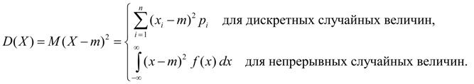(9)

Here m = M(X).

Dispersion properties:

Standard deviation:

(11)

Since the dimension of the standard deviation is the same as that of a random variable, it is more often than the variance used as a measure of dispersion.

distribution moments. The concepts of mathematical expectation and variance are special cases of a more general concept for the numerical characteristics of random variables - distribution moments. The distribution moments of a random variable are introduced as mathematical expectations of some simple functions of a random variable. So, the moment of order k relative to the point X 0 is called expectation M(X–X 0 )k. Moments relative to the origin X= 0 are called initial moments and are marked:

(12)

The initial moment of the first order is the distribution center of the considered random variable:

(13)

Moments relative to distribution center X= m called central points and are marked:

(14)

From (7) it follows that the central moment of the first order is always equal to zero:

The central moments do not depend on the origin of the values ​​of the random variable, since with a shift by a constant value With its center of distribution is shifted by the same value With, and the deviation from the center does not change: X – m = (X – With) – (m – With).
Now it is obvious that dispersion- This second order central moment:

Asymmetry. Central moment of the third order:

(17)

serves to evaluate distribution skewness. If the distribution is symmetrical about the point X= m, then the central moment of the third order will be equal to zero (as well as all central moments of odd orders). Therefore, if the central moment of the third order is different from zero, then the distribution cannot be symmetric. The magnitude of the asymmetry is estimated using a dimensionless asymmetry coefficient:

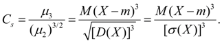(18)

The sign of the asymmetry coefficient (18) indicates right-sided or left-sided asymmetry (Fig. 2).

Rice. 2. Types of asymmetry of distributions.

Excess. Central moment of the fourth order:

(19)

serves to evaluate the so-called kurtosis, which determines the degree of steepness (pointiness) of the distribution curve near the distribution center with respect to the normal distribution curve. Since for a normal distribution, the quantity taken as kurtosis is:

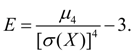(20)

On fig. 3 shows examples of distribution curves with different values ​​of kurtosis. For a normal distribution E= 0. Curves that are more peaked than normal have positive kurtosis, and curves with more flat peaks have negative kurtosis.

Rice. 3. Distribution curves with different degrees of steepness (kurtosis).

Higher-order moments in engineering applications of mathematical statistics are usually not used.

Fashion discrete random variable is its most probable value. Fashion continuous a random variable is its value at which the probability density is maximum (Fig. 2). If the distribution curve has one maximum, then the distribution is called unimodal. If the distribution curve has more than one maximum, then the distribution is called polymodal. Sometimes there are distributions whose curves have not a maximum, but a minimum. Such distributions are called antimodal. In the general case, the mode and the mathematical expectation of a random variable do not coincide. In a particular case, for modal, i.e. having a mode, a symmetric distribution, and provided that there is a mathematical expectation, the latter coincides with the mode and the center of symmetry of the distribution.

Median random variable X is its meaning Me, for which equality holds: i.e. it is equally likely that the random variable X will be less or more Me. Geometrically median is the abscissa of the point at which the area under the distribution curve is divided in half (Fig. 2). In the case of a symmetric modal distribution, the median, mode, and mean are the same.