Mathematical dispersion formula. Dispersion of a discrete random variable

Let's calculate inMSEXCELvariance and standard deviation of the sample. We also calculate the variance of a random variable if its distribution is known.

First consider dispersion, then standard deviation.

Sample variance

Sample variance (sample variance,samplevariance) characterizes the spread of values in the array relative to .

All 3 formulas are mathematically equivalent.

It can be seen from the first formula that sample variance is the sum of the squared deviations of each value in the array from average divided by the sample size minus 1.

dispersion samples the DISP() function is used, eng. the name of the VAR, i.e. VARIance. Since MS EXCEL 2010, it is recommended to use its analogue DISP.V() , eng. the name VARS, i.e. Sample Variance. In addition, starting from the version of MS EXCEL 2010, there is a DISP.G () function, eng. VARP name, i.e. Population VARIance which calculates dispersion for population. The whole difference comes down to the denominator: instead of n-1 like DISP.V() , DISP.G() has just n in the denominator. Prior to MS EXCEL 2010, the VARP() function was used to calculate the population variance.

Sample variance
=SQUARE(Sample)/(COUNT(Sample)-1)
=(SUMSQ(Sample)-COUNT(Sample)*AVERAGE(Sample)^2)/ (COUNT(Sample)-1)- the usual formula
=SUM((Sample -AVERAGE(Sample))^2)/ (COUNT(Sample)-1) –

Sample variance is equal to 0 only if all values are equal to each other and, accordingly, are equal mean value. Usually, the larger the value dispersion, the greater the spread of values in the array.

Sample variance is a point estimate dispersion distribution of the random variable from which the sample. About building confidence intervals when evaluating dispersion can be read in the article.

Variance of a random variable

To calculate dispersion random variable, you need to know it.

For dispersion random variable X often use the notation Var(X). Dispersion is equal to the square of the deviation from the mean E(X): Var(X)=E[(X-E(X)) 2 ]

dispersion calculated by the formula:

where x i is the value that the random variable can take, and μ is the average value (), p(x) is the probability that the random variable will take the value x.

If the random variable has , then dispersion calculated by the formula:

Dimension dispersion corresponds to the square of the unit of measurement of the original values. For example, if the values in the sample are measurements of the weight of the part (in kg), then the dimension of the variance would be kg 2 . This can be difficult to interpret, therefore, to characterize the spread of values, a value equal to the square root of dispersion – standard deviation.

Some properties dispersion:

Var(X+a)=Var(X), where X is a random variable and a is a constant.

Var(aХ)=a 2 Var(X)

Var(X)=E[(X-E(X)) 2 ]=E=E(X 2)-E(2*X*E(X))+(E(X)) 2=E(X 2)- 2*E(X)*E(X)+(E(X)) 2 =E(X 2)-(E(X)) 2

This dispersion property is used in article about linear regression.

Var(X+Y)=Var(X) + Var(Y) + 2*Cov(X;Y), where X and Y are random variables, Cov(X;Y) is the covariance of these random variables.

If random variables are independent, then their covariance is 0, and hence Var(X+Y)=Var(X)+Var(Y). This property of the variance is used in the output.

Let us show that for independent quantities Var(X-Y)=Var(X+Y). Indeed, Var(X-Y)= Var(X-Y)= Var(X+(-Y))= Var(X)+Var(-Y)= Var(X)+Var(-Y)= Var( X)+(-1) 2 Var(Y)= Var(X)+Var(Y)= Var(X+Y). This property of the variance is used to plot .

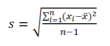
Sample standard deviation

Sample standard deviation is a measure of how widely scattered the values in the sample are relative to their .

A-priory, standard deviation equals the square root of dispersion:

Standard deviation does not take into account the magnitude of the values in sampling, but only the degree of scattering of values around them middle. Let's take an example to illustrate this.

Let's calculate the standard deviation for 2 samples: (1; 5; 9) and (1001; 1005; 1009). In both cases, s=4. It is obvious that the ratio of the standard deviation to the values of the array is significantly different for the samples. For such cases, use The coefficient of variation(Coefficient of Variation, CV) - ratio standard deviation to the average arithmetic, expressed as a percentage.

In MS EXCEL 2007 and earlier versions for calculation Sample standard deviation the function =STDEV() is used, eng. the name STDEV, i.e. standard deviation. Since MS EXCEL 2010, it is recommended to use its analogue = STDEV.B () , eng. name STDEV.S, i.e. Sample STandard DEViation.

In addition, starting from the version of MS EXCEL 2010, there is a function STDEV.G () , eng. name STDEV.P, i.e. Population STandard DEViation which calculates standard deviation for population. The whole difference comes down to the denominator: instead of n-1 like STDEV.V() , STDEV.G() has just n in the denominator.

Standard deviation can also be calculated directly from the formulas below (see example file)
=SQRT(SQUADROTIV(Sample)/(COUNT(Sample)-1))
=SQRT((SUMSQ(Sample)-COUNT(Sample)*AVERAGE(Sample)^2)/(COUNT(Sample)-1))

Other dispersion measures

The SQUADRIVE() function calculates with umm of squared deviations of values from their middle. This function will return the same result as the formula =VAR.G( Sample)*CHECK( Sample) , where Sample- a reference to a range containing an array of sample values (). Calculations in the QUADROTIV() function are made according to the formula:

The SROOT() function is also a measure of the scatter of a set of data. The SIROTL() function calculates the average of the absolute values of the deviations of values from middle. This function will return the same result as the formula =SUMPRODUCT(ABS(Sample-AVERAGE(Sample)))/COUNT(Sample), where Sample- a reference to a range containing an array of sample values.

Calculations in the function SROOTKL () are made according to the formula:

Variation range (or range of variation) - is the difference between the maximum and minimum values of the feature:

In our example, the range of variation in shift output of workers is: in the first brigade R=105-95=10 children, in the second brigade R=125-75=50 children. (5 times more). This suggests that the output of the 1st brigade is more “stable”, but the second brigade has more reserves for the growth of output, because. if all workers reach the maximum output for this brigade, it can produce 3 * 125 = 375 parts, and in the 1st brigade only 105 * 3 = 315 parts.
If the extreme values of the attribute are not typical for the population, then quartile or decile ranges are used. The quartile range RQ= Q3-Q1 covers 50% of the population, the first decile range RD1 = D9-D1 covers 80% of the data, the second decile range RD2= D8-D2 covers 60%.
The disadvantage of the variation range indicator is, but that its value does not reflect all the fluctuations of the trait.
The simplest generalizing indicator that reflects all the fluctuations of a trait is mean linear deviation, which is the arithmetic mean of the absolute deviations of individual options from their average value:

,
for grouped data
,
where хi is the value of the attribute in a discrete series or the middle of the interval in the interval distribution.
In the above formulas, the differences in the numerator are taken modulo, otherwise, according to the property of the arithmetic mean, the numerator will always be equal to zero. Therefore, the average linear deviation is rarely used in statistical practice, only in those cases where summing the indicators without taking into account the sign makes economic sense. With its help, for example, the composition of employees, the profitability of production, and foreign trade turnover are analyzed.
Feature variance is the average square of the deviations of the variant from their average value:
simple variance
,
weighted variance
.
The formula for calculating the variance can be simplified:

Thus, the variance is equal to the difference between the mean of the squares of the variant and the square of the mean of the variant of the population:
.
However, due to the summation of the squared deviations, the variance gives a distorted idea of the deviations, so the average is calculated from it. standard deviation, which shows how much the specific variants of the attribute deviate on average from their average value. Calculated by taking the square root of the variance:
for ungrouped data
,
for the variation series

The smaller the value of the variance and the standard deviation, the more homogeneous the population, the more reliable (typical) the average value will be.
The mean linear and mean square deviation are named numbers, i.e., they are expressed in units of measurement of the attribute, are identical in content and close in value.
It is recommended to calculate the absolute indicators of variation using tables.
Table 3 - Calculation of the characteristics of variation (on the example of the period of data on the shift output of the work teams)

	Number of workers	The middle of the interval	Estimated values
	Number of workers	The middle of the interval




Total:

Average shift output of workers:

Average linear deviation:

Output dispersion:

The standard deviation of the output of individual workers from the average output:
.

1 Calculation of dispersion by the method of moments

The calculation of variances is associated with cumbersome calculations (especially if the average is expressed as a large number with several decimal places). Calculations can be simplified by using a simplified formula and dispersion properties.
The dispersion has the following properties:

if all the values of the attribute are reduced or increased by the same value A, then the variance will not decrease from this:

, then or
Using the properties of the variance and first reducing all the variants of the population by the value A, and then dividing by the value of the interval h, we obtain a formula for calculating the variance in variational series with equal intervals way of moments:
,
where is the dispersion calculated by the method of moments;
h is the value of the interval of the variation series;
– new (transformed) variant values;
A is a constant value, which is used as the middle of the interval with the highest frequency; or the variant with the highest frequency;
is the square of the moment of the first order;
is a moment of the second order.
Let's calculate the variance by the method of moments based on the data on the shift output of the working team.
Table 4 - Calculation of dispersion by the method of moments

Groups of production workers, pcs.	Number of workers	The middle of the interval	Estimated values
Groups of production workers, pcs.	Number of workers	The middle of the interval

Calculation procedure:

calculate the variance:

2 Calculation of the variance of an alternative feature

Among the signs studied by statistics, there are those that have only two mutually exclusive meanings. These are alternative signs. They are given two quantitative values, respectively: options 1 and 0. The frequency of options 1, which is denoted by p, is the proportion of units that have this feature. The difference 1-p=q is the frequency of options 0. Thus,

xi

Arithmetic mean of alternative feature
, since p+q=1.

Feature variance
, because 1-p=q
Thus, the variance of an alternative attribute is equal to the product of the proportion of units that have this attribute and the proportion of units that do not have this attribute.
If the values 1 and 0 are equally frequent, i.e. p=q, the variance reaches its maximum pq=0.25.
Variance variable is used in sample surveys, for example, product quality.

3 Intergroup dispersion. Variance addition rule

Dispersion, unlike other characteristics of variation, is an additive quantity. That is, in the aggregate, which is divided into groups according to the factor criterion X , resultant variance y can be decomposed into variance within each group (within group) and variance between groups (between group). Then, along with the study of the variation of the trait throughout the population as a whole, it becomes possible to study the variation in each group, as well as between these groups.

Total variance measures the variation of a trait at over the entire population under the influence of all the factors that caused this variation (deviations). It is equal to the mean square of the deviations of the individual values of the feature at of the overall mean and can be calculated as simple or weighted variance.
Intergroup variance characterizes the variation of the effective feature at, caused by the influence of the sign-factor X underlying the grouping. It characterizes the variation of the group means and is equal to the mean square of the deviations of the group means from the total mean:
,
where is the arithmetic mean of the i-th group;
– number of units in the i-th group (frequency of the i-th group);
is the total mean of the population.
Intragroup variance reflects random variation, i.e., that part of the variation that is caused by the influence of unaccounted for factors and does not depend on the attribute-factor underlying the grouping. It characterizes the variation of individual values relative to group averages, it is equal to the mean square of deviations of individual values of the trait at within a group from the arithmetic mean of this group (group mean) and is calculated as a simple or weighted variance for each group:
or ,
where is the number of units in the group.
Based on the intra-group variances for each group, it is possible to determine the overall average of the within-group variances:
.
The relationship between the three variances is called variance addition rules, according to which the total variance is equal to the sum of the intergroup variance and the average of the intragroup variances:

Example. When studying the influence of the tariff category (qualification) of workers on the level of productivity of their labor, the following data were obtained.
Table 5 - Distribution of workers by average hourly output.

№ p/n	Workers of the 4th category				Workers of the 5th category
№ p/n	Working out worker, pcs.,				Working out worker, pcs.,
1 2 3 4 5 6	7 9 9 10 12 13	7-10=-3 9-10=-1 -1 0 2 3	9 1 1 0 4 9	1 2 3 4	14 14 15 17	14-15=-1 -1 0 2	1 1 0 4

In this example, the workers are divided into two groups according to the factor X- qualifications, which are characterized by their rank. The effective trait - production - varies both under its influence (intergroup variation) and due to other random factors (intragroup variation). The challenge is to measure these variations using three variances: total, between-group, and within-group. The empirical coefficient of determination shows the proportion of the variation of the resulting feature at under the influence of a factor sign X. The rest of the total variation at caused by changes in other factors.
In the example, the empirical coefficient of determination is:
or 66.7%,
This means that 66.7% of the variation in labor productivity of workers is due to differences in qualifications, and 33.3% is due to the influence of other factors.
Empirical correlation relation shows the tightness of the relationship between the grouping and effective features. It is calculated as the square root of the empirical coefficient of determination:

The empirical correlation ratio , as well as , can take values from 0 to 1.
If there is no connection, then =0. In this case, =0, that is, the group means are equal to each other and there is no intergroup variation. This means that the grouping sign - the factor does not affect the formation of the general variation.
If the relationship is functional, then =1. In this case, the variance of the group means is equal to the total variance (), i.e., there is no intragroup variation. This means that the grouping feature completely determines the variation of the resulting feature being studied.
The closer the value of the correlation relation is to one, the closer, closer to the functional dependence, the relationship between the features.
For a qualitative assessment of the closeness of the connection between the signs, the Chaddock relations are used.

In the example , which indicates a close relationship between the productivity of workers and their qualifications.

Along with the study of the variation of a trait throughout the entire population as a whole, it is often necessary to trace the quantitative changes in the trait in groups into which the population is divided, as well as between groups. This study of variation is achieved by calculating and analyzing various kinds of variance.
Distinguish between total, intergroup and intragroup dispersion.
Total variance σ 2 measures the variation of a trait over the entire population under the influence of all the factors that caused this variation, .

Intergroup variance (δ) characterizes systematic variation, i.e. differences in the magnitude of the trait under study, arising under the influence of the trait-factor underlying the grouping. It is calculated by the formula:
.

Within-group variance (σ) reflects random variation, i.e. part of the variation that occurs under the influence of unaccounted for factors and does not depend on the trait-factor underlying the grouping. It is calculated by the formula:
.

Average of within-group variances: .

There is a law linking 3 types of dispersion. The total variance is equal to the sum of the average of the intragroup and intergroup variances: .
This ratio is called variance addition rule.

In the analysis, a measure is widely used, which is the proportion of between-group variance in the total variance. It bears the name empirical coefficient of determination (η 2): .
The square root of the empirical coefficient of determination is called empirical correlation ratio (η):
.
It characterizes the influence of the attribute underlying the grouping on the variation of the resulting attribute. The empirical correlation ratio varies from 0 to 1.
We will show its practical use in the following example (Table 1).

Example #1. Table 1 - Labor productivity of two groups of workers of one of the workshops of NPO "Cyclone"

Calculate the total and group averages and variances:

The initial data for calculating the average of the intragroup and intergroup dispersion are presented in Table. 2.
table 2
Calculation and δ 2 for two groups of workers.

Worker groups	Number of workers, pers.	Average, det./shift.	Dispersion
Passed technical training	5	95	42,0
Not technically trained	5	81	231,2
All workers	10	88	185,6

Let's calculate the scores. Average of within-group variances:

.
Intergroup variance

Total variance:
Thus, the empirical correlation ratio: .

Along with the variation of quantitative traits, a variation of qualitative traits can also be observed. This study of variation is achieved by calculating the following types of variances:

The intra-group variance of the share is determined by the formula

where n i– the number of units in separate groups.
The proportion of the studied trait in the entire population, which is determined by the formula:
The three types of dispersion are related to each other as follows:

This ratio of variances is called the feature share variance addition theorem.

Probability theory is a special branch of mathematics that is studied only by students of higher educational institutions. Do you love calculations and formulas? Are you not afraid of the prospects of acquaintance with the normal distribution, the entropy of the ensemble, the mathematical expectation and the variance of a discrete random variable? Then this subject will be of great interest to you. Let's get acquainted with some of the most important basic concepts of this section of science.

Let's remember the basics

Even if you remember the simplest concepts of probability theory, do not neglect the first paragraphs of the article. The fact is that without a clear understanding of the basics, you will not be able to work with the formulas discussed below.

So, there is some random event, some experiment. As a result of the actions performed, we can get several outcomes - some of them are more common, others less common. The probability of an event is the ratio of the number of actually obtained outcomes of one type to the total number of possible ones. Only knowing the classical definition of this concept, you can begin to study the mathematical expectation and dispersion of continuous random variables.

Average

Back in school, in mathematics lessons, you started working with the arithmetic mean. This concept is widely used in probability theory, and therefore it cannot be ignored. The main thing for us at the moment is that we will encounter it in the formulas for the mathematical expectation and variance of a random variable.

We have a sequence of numbers and want to find the arithmetic mean. All that is required of us is to sum everything available and divide by the number of elements in the sequence. Let we have numbers from 1 to 9. The sum of the elements will be 45, and we will divide this value by 9. Answer: - 5.

Dispersion

In scientific terms, variance is the average square of the deviations of the obtained feature values from the arithmetic mean. One is denoted by a capital Latin letter D. What is needed to calculate it? For each element of the sequence, we calculate the difference between the available number and the arithmetic mean and square it. There will be exactly as many values as there can be outcomes for the event we are considering. Next, we summarize everything received and divide by the number of elements in the sequence. If we have five possible outcomes, then divide by five.

The variance also has properties that you need to remember in order to apply it when solving problems. For example, if the random variable is increased by X times, the variance increases by X times the square (i.e., X*X). It is never less than zero and does not depend on shifting values by an equal value up or down. Also, for independent trials, the variance of the sum is equal to the sum of the variances.

Now we definitely need to consider examples of the variance of a discrete random variable and the mathematical expectation.

Let's say we run 21 experiments and get 7 different outcomes. We observed each of them, respectively, 1,2,2,3,4,4 and 5 times. What will be the variance?

First, we calculate the arithmetic mean: the sum of the elements, of course, is 21. We divide it by 7, getting 3. Now we subtract 3 from each number in the original sequence, square each value, and add the results together. It turns out 12. Now it remains for us to divide the number by the number of elements, and, it would seem, that's all. But there is a catch! Let's discuss it.

Dependence on the number of experiments

It turns out that when calculating the variance, the denominator can be one of two numbers: either N or N-1. Here N is the number of experiments performed or the number of elements in the sequence (which is essentially the same thing). What does it depend on?

If the number of tests is measured in hundreds, then we must put N in the denominator. If in units, then N-1. The scientists decided to draw the border quite symbolically: today it runs along the number 30. If we conducted less than 30 experiments, then we will divide the amount by N-1, and if more, then by N.

Task

Let's go back to our example of solving the variance and expectation problem. We got an intermediate number of 12, which had to be divided by N or N-1. Since we conducted 21 experiments, which is less than 30, we will choose the second option. So the answer is: the variance is 12 / 2 = 2.

Expected value

Let's move on to the second concept, which we must consider in this article. The mathematical expectation is the result of adding all possible outcomes multiplied by the corresponding probabilities. It is important to understand that the resulting value, as well as the result of calculating the variance, is obtained only once for the whole task, no matter how many outcomes it considers.

The mathematical expectation formula is quite simple: we take the outcome, multiply it by its probability, add the same for the second, third result, etc. Everything related to this concept is easy to calculate. For example, the sum of mathematical expectations is equal to the mathematical expectation of the sum. The same is true for the work. Not every quantity in probability theory allows such simple operations to be performed. Let's take a task and calculate the value of two concepts we have studied at once. In addition, we were distracted by theory - it's time to practice.

One more example

We ran 50 trials and got 10 kinds of outcomes - numbers 0 to 9 - appearing in varying percentages. These are, respectively: 2%, 10%, 4%, 14%, 2%, 18%, 6%, 16%, 10%, 18%. Recall that to get the probabilities, you need to divide the percentage values by 100. Thus, we get 0.02; 0.1 etc. Let us present an example of solving the problem for the variance of a random variable and the mathematical expectation.

We calculate the arithmetic mean using the formula that we remember from elementary school: 50/10 = 5.

Now let's translate the probabilities into the number of outcomes "in pieces" to make it more convenient to count. We get 1, 5, 2, 7, 1, 9, 3, 8, 5 and 9. Subtract the arithmetic mean from each value obtained, after which we square each of the results obtained. See how to do this with the first element as an example: 1 - 5 = (-4). Further: (-4) * (-4) = 16. For other values, do these operations yourself. If you did everything right, then after adding everything you get 90.

Let's continue calculating the variance and mean by dividing 90 by N. Why do we choose N and not N-1? That's right, because the number of experiments performed exceeds 30. So: 90/10 = 9. We got the dispersion. If you get a different number, don't despair. Most likely, you made a banal error in the calculations. Double-check what you wrote, and for sure everything will fall into place.

Finally, let's recall the mathematical expectation formula. We will not give all the calculations, we will only write the answer with which you can check after completing all the required procedures. The expected value will be 5.48. We only recall how to carry out operations, using the example of the first elements: 0 * 0.02 + 1 * 0.1 ... and so on. As you can see, we simply multiply the value of the outcome by its probability.

Deviation

Another concept closely related to dispersion and mathematical expectation is the standard deviation. It is denoted either by the Latin letters sd, or by the Greek lowercase "sigma". This concept shows how, on average, values deviate from the central feature. To find its value, you need to calculate the square root of the variance.

If you plot a normal distribution and want to see the squared deviation directly on it, this can be done in several steps. Take half of the image to the left or right of the mode (central value), draw a perpendicular to the horizontal axis so that the areas of the resulting figures are equal. The value of the segment between the middle of the distribution and the resulting projection on the horizontal axis will be the standard deviation.

Software

As can be seen from the descriptions of the formulas and the examples presented, calculating the variance and mathematical expectation is not the easiest procedure from an arithmetic point of view. In order not to waste time, it makes sense to use the program used in higher education - it is called "R". It has functions that allow you to calculate values for many concepts from statistics and probability theory.

For example, you define a vector of values. This is done as follows: vector<-c(1,5,2…). Теперь, когда вам потребуется посчитать какие-либо значения для этого вектора, вы пишете функцию и задаете его в качестве аргумента. Для нахождения дисперсии вам нужно будет использовать функцию var. Пример её использования: var(vector). Далее вы просто нажимаете «ввод» и получаете результат.

Finally

Dispersion and mathematical expectation are without which it is difficult to calculate anything in the future. In the main course of lectures at universities, they are considered already in the first months of studying the subject. It is precisely because of the lack of understanding of these simple concepts and the inability to calculate them that many students immediately begin to fall behind in the program and later receive poor marks in the session, which deprives them of scholarships.

Practice at least one week for half an hour a day, solving tasks similar to those presented in this article. Then, on any probability theory test, you will cope with examples without extraneous tips and cheat sheets.

The main generalizing indicators of variation in statistics are dispersion and standard deviation.

Dispersion it arithmetic mean squared deviations of each feature value from the total mean. The variance is usually called the mean square of the deviations and is denoted  2 . Depending on the initial data, the variance can be calculated from the arithmetic mean, simple or weighted:

 unweighted (simple) dispersion;

 weighted variance.

Standard deviation is a generalizing characteristic of absolute dimensions variations trait in the aggregate. It is expressed in the same units as the sign (in meters, tons, percent, hectares, etc.).

The standard deviation is the square root of the variance and is denoted by :

 unweighted standard deviation;

 weighted standard deviation.

The standard deviation is a measure of the reliability of the mean. The smaller the standard deviation, the better the arithmetic mean reflects the entire represented population.

The calculation of the standard deviation is preceded by the calculation of the variance.

The procedure for calculating the weighted variance is as follows:

1) determine the arithmetic weighted average:

2) calculate the deviations of the options from the average:

3) square the deviation of each option from the mean:

4) multiply the squared deviations by the weights (frequencies):

5) summarize the received works:

6) the resulting amount is divided by the sum of the weights:

Example 2.1

Calculate the arithmetic weighted average:

The values of deviations from the mean and their squares are presented in the table. Let's define the variance:

The standard deviation will be equal to:

If the source data is presented as an interval distribution series , then you first need to determine the discrete value of the feature, and then apply the method described.

Example 2.2

Let us show the calculation of the variance for the interval series on the data on the distribution of the sown area of the collective farm by wheat yield.

The arithmetic mean is:

Let's calculate the variance:

6.3. Calculation of the dispersion according to the formula for individual data

Calculation technique dispersion complex, and for large values of options and frequencies can be cumbersome. Calculations can be simplified using the dispersion properties.

The dispersion has the following properties.

1. A decrease or increase in the weights (frequencies) of a variable feature by a certain number of times does not change the dispersion.

2. Decreasing or increasing each feature value by the same constant value BUT dispersion does not change.

3. Decreasing or increasing each feature value by a certain number of times k respectively reduces or increases the variance in k 2 times standard deviation  in k once.

4. The variance of a feature relative to an arbitrary value is always greater than the variance relative to the arithmetic mean by the square of the difference between the average and arbitrary values:

If a BUT 0, then we arrive at the following equality:

i.e., the variance of a feature is equal to the difference between the mean square of the feature values and the square of the mean.

Each property can be used alone or in combination with others when calculating the variance.

The procedure for calculating the variance is simple:

1) determine arithmetic mean :

2) square the arithmetic mean:

3) square the deviation of each variant of the series:

X i 2 .

4) find the sum of squares of options:

5) divide the sum of squares of options by their number, i.e. determine the average square:

6) determine the difference between the mean square of the feature and the square of the mean:

Example 3.1 We have the following data on the productivity of workers:

Let's make the following calculations: