Solving equations by simple iteration excel. List of used literary sources

Excel has a wide range of tools for solving different types of equations using different methods.

Let's look at some examples of solutions.

Solving equations by the method of selecting Excel parameters

The Parameter Seek tool is used in a situation where the result is known, but the arguments are unknown. Excel picks values until the calculation yields the desired total.

Path to the command: "Data" - "Working with data" - "What-if analysis" - "Parameter selection".

Consider, for example, the solution of the quadratic equation x 2 + 3x + 2 = 0. The order of finding the root using Excel:

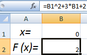
The program uses a cyclic process to select the parameter. To change the number of iterations and the error, you need to go to the Excel options. On the "Formulas" tab, set the maximum number of iterations, the relative error. Check the box "enable iterative calculations".

How to solve system of equations by matrix method in Excel

The system of equations is given:

Equation roots are obtained.

Solving a system of equations by Cramer's method in Excel

Let's take the system of equations from the previous example:

To solve them by the Cramer method, we calculate the determinants of the matrices obtained by replacing one column in matrix A with a column-matrix B.

To calculate the determinants, we use the MOPRED function. The argument is a range with the corresponding matrix.

We also calculate the determinant of matrix A (array - range of matrix A).

The determinant of the system is greater than 0 - the solution can be found using the Cramer formula (D x / |A|).

To calculate X 1: \u003d U2 / $ U $ 1, where U2 - D1. To calculate X 2: =U3/$U$1. Etc. We get the roots of the equations:

Solving systems of equations by the Gauss method in Excel

For example, let's take the simplest system of equations:

3a + 2c - 5c = -1
2a - c - 3c = 13
a + 2b - c \u003d 9

We write the coefficients in matrix A. Free terms - in matrix B.

For clarity, we highlight the free members by filling. If there is 0 in the first cell of matrix A, you need to swap the rows so that there is a value other than 0 here.

Examples of solving equations by iteration in Excel

The calculations in the workbook must be set up as follows:

This is done on the "Formulas" tab in the "Excel Options". Let's find the root of the equation x - x 3 + 1 = 0 (a = 1, b = 2) by iteration using cyclic references. Formula:

X n+1 \u003d X n - F (X n) / M, n \u003d 0, 1, 2, ....

M is the maximum value of the modulo derivative. To find M, let's do the calculations:

f' (1) = -2 * f' (2) = -11.

The resulting value is less than 0. Therefore, the function will be with the opposite sign: f (x) \u003d -x + x 3 - 1. M \u003d 11.

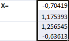
In cell A3, enter the value: a = 1. Accuracy - three decimal places. To calculate the current value of x in the adjacent cell (B3), enter the formula: =IF(B3=0;A3;B3-(-B3+POWER(B3;3)-1/11)).

In cell C3, we control the value of f (x): using the formula =B3-POWER(B3;3)+1.

The root of the equation is 1.179. Enter the value 2 in cell A3. We get the same result:

There is only one root on a given interval.

Finding the roots of equations

The graphical way to find the roots is to plot the function f (x) on the segment. The point of intersection of the graph of the function with the abscissa axis gives an approximate value of the root of the equation.

The approximate values of the roots found in this way make it possible to single out segments on which, if necessary, it is possible to refine the roots.

When finding roots by calculation for continuous functions f(x), the following considerations are used:

- if the function has different signs at the ends of the segment, then there is an odd number of roots between the points a and b on the x-axis;

- if the function has the same signs at the ends of the interval, then between a and b there is an even number of roots or there are none at all;

- if the function has different signs at the ends of the segment and either the first derivative or the second derivative do not change signs on this segment, then the equation has a single root on the segment.

Find all real roots of the equation x 5 –4x–2=0 on the segment [–2,2]. Let's create a spreadsheet.

Table 1

Table 2 shows the calculation results.

table 2

Similarly, a solution is found on the intervals [-2,-1], [-1,0].

Refinement of the roots of the equation

Using the "Search for solutions" mode

For the equation given above, all roots of the equation x 5 –4x–2=0 should be clarified with an error of E = 0.001.

To clarify the roots in the interval [-2,-1], we will compile a spreadsheet.

Table 3

We start the "Search for a solution" mode in the "Tools" menu. Execute mode commands. The display mode will display the found roots. Similarly, we refine the roots on other intervals.

Refinement of Equation Roots

Using the "Iterations" mode

The simple iteration method has two modes "Manual" and "Automatic". To start the "Iterations" mode in the "Tools" menu, open the "Parameters" tab. The following are the mode commands. On the Calculations tab, you can select automatic or manual mode.

Solving systems of equations

The solution of systems of equations in Excel is carried out by the method of inverse matrices. Solve the system of equations:

Let's create a spreadsheet.

Table 4

A	B	C	D	E
Solution of the system of equations.

	ax=b

Initial matrix A		Right side b
-8
		-3
		-2		-2

Inverse Matrix (1/A)		Solution vector x=(1/A)/b
=MOBR(A6:C8)	=MOBR(A6:C8)	=MOBR(A6:C8)		=MULTI(A11:C13,E6:E8)
=MOBR(A6:C8)	=MOBR(A6:C8)	=MOBR(A6:C8)		=MULTI(A11:C13,E6:E8)
=MOBR(A6:C8)	=MOBR(A6:C8)	=MOBR(A6:C8)		=MULTI(A11:C13,E6:E8)

The MIN function returns an array of values that is inserted into an entire column of cells at once.

Table 5 presents the calculation results.

Table 5

A	B	C	D	E
Solution of the system of equations.

	ax=b

Initial matrix A		Right side b
-8
		-3
		-2		-2

Inverse Matrix (1/A)		Solution vector x=(1/A)/b
-0,149	0,054	-0,230
0,054	0,162	-0,189
-0,122	0,135	-0,824

List of used literary sources

1. Turchak L.I. Fundamentals of numerical methods: Proc. allowance for universities / ed. V.V. Shchennikov.–M.: Nauka, 1987.–320p.

2. Bundy B. Optimization methods. Introductory course.–M.: Radio and communication, 1988.–128s.

3. Evseev A.M., Nikolaeva L.S. Mathematical modeling of chemical equilibria.–M.: Izd-vo Mosk. un-ta, 1988.–192p.

4. Bezdenezhnykh A.A. Engineering methods for compiling reaction rate equations and calculating kinetic constants.–L.: Chemistry, 1973.–256p.

5. Stepanova N.F., Erlykina M.E., Filippov G.G. Methods of linear algebra in physical chemistry.–M.: Izd-vo Mosk. un-ta, 1976.–359p.

6. Bakhvalov N.S. and others. Numerical methods in tasks and exercises: Proc. manual for universities / Bakhvalov N.S., Lapin A.V., Chizhonkov E.V. - M.: Higher. school., 2000.-190s. - (Higher mathematics / Sadovnichiy V.A.)

7. Application of Computational Mathematics in Chemical and Physical Kinetics, ed. L.S. Polak, M.: Nauka, 1969, 279 pp.

8. Algorithmization of calculations in chemical technology B.A. Zhidkov, A.G. Cooper

9. Computational methods for chemical engineers. H. Rosenbrock, S. Story

10. Orvis V.D. Excel for scientists, engineers and students. - Kyiv: Junior, 1999.

11. Yu.Yu. Tarasevich Numerical methods at Mathcade - Astrakhan State Pedagogical University: Astrakhan, 2000.

Example 3.1 . Find a solution to the system of linear algebraic equations (3.1) using the Jacobi method.

Iterative methods can be used for a given system, because the condition "predominance of diagonal coefficients", which ensures the convergence of these methods.

The design scheme of the Jacobi method is shown in Figure (3.1).

Bring the system (3.1). to normal view:

, (3.2)

or in matrix form

, (3.3)

Fig.3.1.

To determine the number of iterations required to achieve a given accuracy e, and an approximate solution of the system is useful in the column H install Conditional Format. The result of such formatting is visible in Figure 3.1. Column cells H, whose values satisfy condition (3.4) are shaded.

(3.4)

Analyzing the results, we take the fourth iteration as an approximate solution of the original system with a given accuracy e=0.1,

those. x 1=10216; x 2= 2,0225, x 3= 0,9912

Changing the value e in a cell H5 it is possible to obtain a new approximate solution of the original system with a new accuracy.

Analyze the convergence of the iterative process by plotting changes in each component of the SLAE solution depending on the iteration number.

To do this, select a block of cells A10:D20 and using Chart Wizard, build graphs that reflect the convergence of the iterative process, Fig.3.2.

The system of linear algebraic equations is solved similarly by the Seidel method.

Lab #4

Subject. Numerical methods for solving linear ordinary differential equations with boundary conditions. Finite difference method

Exercise. Solve the boundary value problem by the finite difference method by constructing two approximations (two iterations) with step h and step h/2.

Analyze the results. Task options are given in Appendix 4.

Work order

1. Build manually finite difference approximation of the boundary value problem (finite difference SLAE) with step h , given option.

2. Using the finite difference method, form in excel system of linear algebraic finite-difference equations for the step h segment breakdown . Record this SLAE on the worksheet of the book. excel. The design scheme is shown in Figure 4.1.

3. Solve the resulting SLAE by the sweep method.

4. Check the correctness of the SLAE solution using the add-on Excel Find solution.

5. Reduce the grid step by 2 times and solve the problem again. Present the results graphically.

6. Compare your results. Make a conclusion about the need to continue or terminate the account.

Solving a boundary value problem using Microsoft Excel spreadsheets.

Example 4.1. Using the finite difference method to find a solution to the boundary value problem , y(1)=1, y’(2)=0.5 on the segment xО with step h=0.2 and with step h=0.1. Compare the results and draw a conclusion about the need to continue or terminate the account.

The calculation scheme for step h=0.2 is shown in Fig.4.1.

The resulting solution (grid function) Y {1.000, 1.245, 1.474, 1.673, 1.829, 1.930}, X (1; 1.2; 1.4; 1.6; 1.8; 2) in columns L and B can be taken as the first iteration (first approximation) of the original problem.

For finding second iteration make the grid twice as thick (n=10, stride h=0.1) and repeat the above algorithm.

This can be done on the same or on another sheet of the book. excel. The solution (second approximation) is shown in Figure 4.2.

Compare the obtained approximate solutions. For clarity, you can build graphs of these two approximations (two grid functions), Fig.4.3.

The procedure for constructing graphs of approximate solutions to a boundary value problem

1. Build a graph for solving the problem for a difference grid with a step h=0.2 (n=5).

2. Activate the already built chart and select the command menu Chart\Add Data

3. In the window New data enter data x i , y i for difference grid with step h/2 (n=10).

4. In the window Special insert check the boxes in the fields:

Ø new rows,

As can be seen from the data presented, two approximate solutions of the boundary value problem (two grid functions) differ from each other by no more than 5%. Therefore, we take the second iteration as an approximate solution of the original problem, i.e.

Y{1, 1.124, 1.246, 1.364, 1.478, 1.584, 1.683, 1.772, 1.849, 1.914, 1.964}

Lab #5

Ministry of General Education

Russian Federation

Ural State Technical University-UPI

branch in Krasnoturinsk

Department of Computer Engineering

Course work

By numerical methods

Solving linear equations by simple iteration

using Microsoft Excel

Head Kuzmina N.V.

Student Nigmatzyanov T.R.

Group M-177T

Topic: "Finding with a given accuracy the root of the equation F(x)=0 on the interval by the method of simple iteration."

Test Case: 0.25-x+sinx=0

Conditions of the problem: for a given function F(x) on the interval, find the root of the equation F(x)=0 by simple iteration.

The root is calculated twice (using automatic and manual calculation).

Provide for the construction of a graph of a function at a given interval.

Introduction 4

1. Theoretical part 5

2. Description of the progress of work 7

3.Input and output data 8

Conclusion 9

Annex 10

References 12

Introduction.

In the course of this work, I need to get acquainted with various methods for solving the equation and find the root of the non-linear equation 0.25-x + sin (x) \u003d 0 by a numerical method - the method of simple iteration. To check the correctness of finding the root, it is necessary to solve the equation graphically, find an approximate value and compare it with the result obtained.

1. Theoretical part.

Simple iteration method.

The iterative process consists in successive refinement of the initial approximation x0 (the root of the equation). Each such step is called an iteration.

To use this method, the original nonlinear equation is written as: x=j(x), i.e. x stands out; j(х) is continuous and differentiable on the interval (a; c). This can usually be done in several ways:

For example:

arcsin(2x+1)-x 2 =0 (f(x)=0)

Method 1.

arcsin(2x+1)=x2

sin(arcsin(2x+1))=sin(x2)

x=0.5(sinx 2 -1) (x=j(x))

Method 2.

x=x+arcsin(2x+1)-x 2 (x=j(x))

Method 3.

x 2 =arcsin(2x+1)

x= (x=j(x)), the sign is taken depending on the interval [a;b].

The transformation must be such that ½j(x)<1½ для всех принадлежащих интервалу .В таком случае процесс итерации сходится.

Let the initial approximation of the root x \u003d c 0 be known. Substituting this value into the right side of the equation x \u003d j (x), we obtain a new approximation of the root: c \u003d j (c 0). x), we get a sequence of values

c n =j(c n-1) n=1,2,3,…

The iteration process should be continued until the following condition is met for two successive approximations: ½c n -c n -1 ½

You can solve equations numerically using programming languages, but Excel makes it possible to cope with this task in a simpler way.

Excel implements the simple iteration method in two ways, with manual calculation and with automatic precision control.

y y=x

j (from 0)

s 0 s 2 s 4 s 6 s 8 root s 9 s 7 s 5 s 3 s 1

Rice. Iterative Process Graph

2. Description of the progress of work.

1. Launched ME.

2. I built a graph of the function y=x and y=0.25+sin(x) on a segment with a step of 0.1 called the sheet "Graph".

3. Chose a team Service ® Options.
Opened a tab Computing .
Turned on the mode Manually .
Disabled checkbox Recalculation before saving . Made the field value Limit number of iterations equal to 1, the relative error is 0.001.

4. Entered in cell A1 the line "Solution of the equation x = 0.25 + sin (x) by the method of simple iteration."

5. Entered the text “Initial value” in cell A3, the text “Initial flag” in cell A4, the value 0.5 in cell B3, the word TRUE in cell B4.

6. Assigned to cells B3 and B4 the name "start_value" and "start".
Cell B6 will check to see if true is equal to the value of cell "begin". 0.25 + sine x. In cell B7, the 0.25-sine of cell B6 is calculated, and thus a cyclic reference is organized.

7. In cell A6 entered y=x, and in cell A7 y=0.25+sin(x). In cell B6 the formula:
=IF(start,start_value,B7).
In cell B7 formula: y=0.25+sin(B6).

8. In cell A9 entered the word Error.

9. In cell B9 I entered the formula: \u003d B7-B6.

10. Using the command Format-Cells (tab Number ) converted cell B9 to exponential format with two decimal places.

11. Then I organized a second cyclic link for counting the number of iterations. In cell A11 I entered the text “Number of iterations”.

12. In cell B11, I entered the formula: \u003d IF (beginning; 0; B12 + 1).

13. In cell B12 entered =B11.

14. To perform the calculation, set the table cursor in cell B4 and pressed the F9 (Calculate) key to start solving the problem.

15. Changed the value of the initial flag to FALSE, and pressed F9 again. Each time F9 is pressed, one iteration is performed and the next approximate value of x is calculated.

16. Pressed the F9 key until the x value reached the required accuracy.
With automatic calculation:

17. Moved to another sheet.

18. I repeated points 4 to 7, only in cell B4 I entered the value FALSE.

19. Chose a team Service ® Options (tab Computing ).Set the value of the field Limit number of iterations equal to 100, relative error equal to 0.0000001. Automatically .