Standard deviation formula. How to calculate standard deviation? Dispersion

The most perfect characteristic of variation is the standard deviation, which is called the standard (or standard deviation). Standard deviation() is equal to the square root of the mean square of the deviations of individual feature values from the arithmetic mean:

The standard deviation is simple:

The weighted standard deviation is applied for grouped data:

Between the mean square and mean linear deviations under conditions of normal distribution, the following relationship takes place: ~ 1.25.

The standard deviation, being the main absolute measure of variation, is used in determining the values of the ordinates of the normal distribution curve, in calculations related to the organization of sample observation and establishing the accuracy of sample characteristics, as well as in assessing the boundaries of the variation of a trait in a homogeneous population.

Dispersion, its types, standard deviation.

Variance of a random variable- a measure of the spread of a given random variable, i.e., its deviation from the mathematical expectation. In statistics, the designation or is often used. The square root of the variance is called the standard deviation, standard deviation, or standard spread.

Total variance (σ2) measures the variation of a trait in the entire population under the influence of all the factors that caused this variation. At the same time, thanks to the grouping method, it is possible to isolate and measure the variation due to the grouping feature, and the variation that occurs under the influence of unaccounted for factors.

Intergroup variance (σ 2 m.gr) characterizes systematic variation, i.e., differences in the magnitude of the studied trait arising under the influence of the trait - the factor underlying the grouping.

standard deviation(synonyms: standard deviation, standard deviation, standard deviation; similar terms: standard deviation, standard spread) - in probability theory and statistics, the most common indicator of the dispersion of the values of a random variable relative to its mathematical expectation. With limited arrays of samples of values, instead of the mathematical expectation, the arithmetic mean of the set of samples is used.

The standard deviation is measured in units of the random variable itself and is used in calculating the standard error of the arithmetic mean, in constructing confidence intervals, in statistical testing of hypotheses, and in measuring the linear relationship between random variables. It is defined as the square root of the variance of a random variable.

Standard deviation:

Standard deviation(estimation of the standard deviation of a random variable x relative to its mathematical expectation based on an unbiased estimate of its variance):

where is the dispersion; — i-th sample element; — sample size; - arithmetic mean of the sample:

It should be noted that both estimates are biased. In the general case, it is impossible to construct an unbiased estimate. However, an estimate based on an unbiased variance estimate is consistent.

Essence, scope and procedure for determining the mode and median.

In addition to power-law averages in statistics, for a relative characteristic of the magnitude of a varying trait and the internal structure of distribution series, structural averages are used, which are mainly represented by mode and median.

Fashion- This is the most common variant of the series. Fashion is used, for example, in determining the size of clothes, shoes, which are in greatest demand among buyers. The mode for a discrete series is the variant with the highest frequency. When calculating the mode for the interval variation series, you must first determine the modal interval (by the maximum frequency), and then the value of the modal value of the attribute according to the formula:

- - fashion value

- - lower limit of the modal interval

- - interval value

- - modal interval frequency

- - frequency of the interval preceding the modal

- - frequency of the interval following the modal

Median - this is the value of the feature that underlies the ranked series and divides this series into two parts equal in number.

To determine the median in a discrete series in the presence of frequencies, first calculate the half-sum of frequencies , and then determine what value of the variant falls on it. (If the sorted row contains an odd number of features, then the median number is calculated by the formula:

M e \u003d (n (number of features in the aggregate) + 1) / 2,

in the case of an even number of features, the median will be equal to the average of the two features in the middle of the row).

When calculating medians for an interval variation series, first determine the median interval within which the median is located, and then the value of the median according to the formula:

- is the desired median

- is the lower bound of the interval that contains the median

- - interval value

- - the sum of the frequencies or the number of members of the series

The sum of the accumulated frequencies of the intervals preceding the median

- is the frequency of the median interval

Example. Find the mode and median.

Decision:
In this example, the modal interval is within the age group of 25-30 years, since this interval accounts for the highest frequency (1054).

Let's calculate the mode value:

This means that the modal age of students is 27 years.

Calculate the median. The median interval is in the age group of 25-30 years, since within this interval there is a variant that divides the population into two equal parts (Σf i /2 = 3462/2 = 1731). Next, we substitute the necessary numerical data into the formula and get the value of the median:

This means that one half of the students are under 27.4 years old, and the other half are over 27.4 years old.

In addition to the mode and median, indicators such as quartiles can be used, dividing the ranked series into 4 equal parts, deciles- 10 parts and percentiles - per 100 parts.

The concept of selective observation and its scope.

Selective observation applies when applying continuous observation physically impossible due to a large amount of data or economically impractical. Physical impossibility occurs, for example, when studying passenger flows, market prices, family budgets. Economic inexpediency occurs when assessing the quality of goods associated with their destruction, for example, tasting, testing bricks for strength, etc.

Statistical units selected for observation make up a sample or sample, and their entire array - the general population (GS). In this case, the number of units in the sample denotes n, and in the entire HS - N. Attitude n/n called the relative size or proportion of the sample.

The quality of the sampling results depends on the representativeness of the sample, i.e. how representative it is in the HS. To ensure the representativeness of the sample, it is necessary to observe principle of random selection of units, which assumes that the inclusion of a HS unit in the sample cannot be influenced by any other factor than chance.

Exist 4 ways of random selection to sample:

Actually random selection or "lotto method", when serial numbers are assigned to statistical values, entered on certain objects (for example, kegs), which are then mixed in some container (for example, in a bag) and selected at random. In practice, this method is carried out using a random number generator or mathematical tables of random numbers.
Mechanical selection, according to which each ( N/n)-th value of the general population. For example, if it contains 100,000 values, and you want to select 1,000, then every 100,000 / 1000 = 100th value will fall into the sample. Moreover, if they are not ranked, then the first one is chosen at random from the first hundred, and the numbers of the others will be one hundred more. For example, if unit number 19 was the first, then number 119 should be next, then number 219, then number 319, and so on. If the population units are ranked, then #50 is selected first, then #150, then #250, and so on.
The selection of values from a heterogeneous data array is carried out stratified(stratified) method, when the general population is previously divided into homogeneous groups, to which random or mechanical selection is applied.
A special sampling method is serial selection, in which not individual quantities are randomly or mechanically chosen, but their series (sequences from some number to some consecutive), within which continuous observation is carried out.

The quality of sample observations also depends on sampling type: repeated or non-repetitive.

At re-selection the statistical values or their series that fell into the sample are returned to the general population after use, having a chance to get into a new sample. At the same time, all values of the general population have the same probability of being included in the sample.

Non-repeating selection means that the statistical values or their series included in the sample are not returned to the general population after use, and therefore the probability of getting into the next sample increases for the remaining values of the latter.

Non-repetitive sampling gives more accurate results, so it is used more often. But there are situations when it cannot be applied (study of passenger flows, consumer demand, etc.) and then a re-selection is carried out.

The marginal error of the observation sample, the average error of the sample, the order in which they are calculated.

Let us consider in detail the above methods of forming a sample population and the errors that arise in this case. representativeness .
Actually-random the sample is based on the selection of units from the general population at random without any elements of consistency. Technically, proper random selection is carried out by drawing lots (for example, lotteries) or by a table of random numbers.

Actually-random selection "in its pure form" in the practice of selective observation is rarely used, but it is the initial among other types of selection, it implements the basic principles of selective observation. Let us consider some questions of the theory of the sampling method and the error formula for a simple random sample.

Sampling error- this is the difference between the value of the parameter in the general population, and its value calculated from the results of sample observation. For an average quantitative characteristic, the sampling error is determined by

The indicator is called the marginal sampling error.
The sample mean is a random variable that can take on different values depending on which units are in the sample. Therefore, sampling errors are also random variables and can take on different values. Therefore, determine the average of the possible errors - mean sampling error, which depends on:

Sample size: the larger the number, the smaller the average error;

The degree of change of the studied trait: the smaller the variation of the trait, and, consequently, the variance, the smaller the average sampling error.

At random re-selection the average error is calculated:
.
In practice, the general variance is not exactly known, but in probability theory proved that
.
Since the value for sufficiently large n is close to 1, we can assume that . Then the mean sampling error can be calculated:
.
But in cases of a small sample (for n<30) коэффициент необходимо учитывать, и среднюю ошибку малой выборки рассчитывать по формуле
.

At random sampling the given formulas are corrected by the value . Then the average error of non-sampling is:
and .
Because is always less than , then the factor () is always less than 1. This means that the average error in non-repetitive selection is always less than in repeated selection.
Mechanical sampling is used when the general population is ordered in some way (for example, voter lists in alphabetical order, telephone numbers, house numbers, apartments). The selection of units is carried out at a certain interval, which is equal to the reciprocal of the percentage of the sample. So, with a 2% sample, every 50 unit = 1 / 0.02 is selected, with 5%, each 1 / 0.05 = 20 unit of the general population.

The origin is chosen in different ways: randomly, from the middle of the interval, with a change in the origin. The main thing is to avoid systematic error. For example, with a 5% sample, if the 13th is chosen as the first unit, then the next 33, 53, 73, etc.

In terms of accuracy, mechanical selection is close to proper random sampling. Therefore, to determine the average error of mechanical sampling, formulas of proper random selection are used.

At typical selection the surveyed population is preliminarily divided into homogeneous, single-type groups. For example, when surveying enterprises, these can be industries, sub-sectors, while studying the population - areas, social or age groups. Then an independent selection is made from each group in a mechanical or proper random way.

Typical sampling gives more accurate results than other methods. The typification of the general population ensures the representation of each typological group in the sample, which makes it possible to exclude the influence of intergroup variance on the average sample error. Therefore, when finding the error of a typical sample according to the rule of addition of variances (), it is necessary to take into account only the average of the group variances. Then the mean sampling error is:
in re-selection
,
with non-recurring selection
,
where is the mean of the intra-group variances in the sample.

Serial (or nested) selection used when the population is divided into series or groups before the start of the sample survey. These series can be packages of finished products, student groups, teams. Series for examination are selected mechanically or randomly, and within the series a complete survey of units is carried out. Therefore, the average sampling error depends only on the intergroup (interseries) variance, which is calculated by the formula:

where r is the number of selected series;
- the average of the i-th series.

The average serial sampling error is calculated:

when reselected:
,
with non-recurring selection:
,
where R is the total number of series.

Combined selection is a combination of the considered methods of selection.

The average sampling error for any selection method depends mainly on the absolute size of the sample and, to a lesser extent, on the percentage of the sample. Suppose that 225 observations are made in the first case out of a population of 4,500 units and in the second case, out of 225,000 units. The variances in both cases are equal to 25. Then, in the first case, with a 5% selection, the sampling error will be:

In the second case, with a 0.1% selection, it will be equal to:

Thus, with a decrease in the sample percentage by 50 times, the sample error increased slightly, since the sample size did not change.
Assume that the sample size is increased to 625 observations. In this case, the sampling error is:

An increase in the sample by 2.8 times with the same size of the general population reduces the size of the sampling error by more than 1.6 times.

Methods and means of forming a sample population.

In statistics, various methods of forming sample sets are used, which is determined by the objectives of the study and depends on the specifics of the object of study.

The main condition for conducting a sample survey is to prevent the occurrence of systematic errors arising from the violation of the principle of equal opportunities for each unit of the general population to enter the sample. The prevention of systematic errors is achieved as a result of the use of scientifically based methods for the formation of a sample population.

There are the following ways to select units from the general population:

1) individual selection - individual units are selected in the sample;

2) group selection - qualitatively homogeneous groups or series of units under study fall into the sample;

3) combined selection is a combination of individual and group selection.
Methods of selection are determined by the rules for the formation of the sampling population.

The sample can be:

proper random consists in the fact that the sample is formed as a result of random (unintentional) selection of individual units from the general population. In this case, the number of units selected in the sample set is usually determined based on the accepted proportion of the sample. The sample share is the ratio of the number of units in the sample population n to the number of units in the general population N, i.e.

mechanical consists in the fact that the selection of units in the sample is made from the general population, divided into equal intervals (groups). In this case, the size of the interval in the general population is equal to the reciprocal of the proportion of the sample. So, with a 2% sample, every 50th unit is selected (1:0.02), with a 5% sample, every 20th unit (1:0.05), etc. Thus, in accordance with the accepted proportion of selection, the general population is, as it were, mechanically divided into equal groups. Only one unit is selected from each group in the sample.
typical - in which the general population is first divided into homogeneous typical groups. Then, from each typical group, an individual selection of units into the sample is made by a proper random or mechanical sample. An important feature of a typical sample is that it gives more accurate results compared to other methods of selecting units in a sample;
serial- in which the general population is divided into groups of the same size - series. Series are selected in the sample set. Within the series, a continuous observation of the units that fell into the series is carried out;
combined- sampling can be two-stage. In this case, the general population is first divided into groups. Then the groups are selected, and within the latter, individual units are selected.

In statistics, the following methods of selecting units in a sample are distinguished::

single stage sample - each selected unit is immediately subjected to study on a given basis (actually random and serial samples);
multistage sampling - selection is made from the general population of individual groups, and individual units are selected from the groups (a typical sample with a mechanical method of selecting units in the sample population).

In addition, there are:

reselection- according to the scheme of the returned ball. In this case, each unit or series that has fallen into the sample is returned to the general population and therefore has a chance to be included in the sample again;
non-repetitive selection- according to the scheme of the unreturned ball. It has more accurate results for the same sample size.

Determination of the required sample size (using Student's table).

One of the scientific principles in sampling theory is to ensure that a sufficient number of units are selected. Theoretically, the need to comply with this principle is presented in the proofs of the limit theorems of probability theory, which allow you to establish how many units should be selected from the general population so that it is sufficient and ensures the representativeness of the sample.

A decrease in the standard error of the sample, and, consequently, an increase in the accuracy of the estimate is always associated with an increase in the sample size, therefore, already at the stage of organizing a sample observation, it is necessary to decide what the sample size should be in order to ensure the required accuracy of the observation results. The calculation of the required sample size is built using formulas derived from the formulas for the marginal sampling errors (A), corresponding to one or another type and method of selection. So, for a random repeated sample size (n), we have:

The essence of this formula is that with a random re-selection of the required number, the sample size is directly proportional to the square of the confidence coefficient (t2) and variance of the variation feature (?2) and is inversely proportional to the square of the marginal sampling error (?2). In particular, by doubling the marginal error, the required sample size can be reduced by a factor of four. Of the three parameters, two (t and?) are set by the researcher.

At the same time, the researcher For the purposes of the sample survey, the question should be decided: in what quantitative combination is it better to include these parameters in order to provide the optimal variant? In one case, he may be more satisfied with the reliability of the results obtained (t) than with the measure of accuracy (?), in the other - vice versa. It is more difficult to resolve the issue regarding the value of the marginal sampling error, since the researcher does not have this indicator at the stage of designing a sample observation, therefore, in practice, it is customary to set the marginal sampling error, as a rule, within 10% of the expected average level of the trait. Establishing an assumed average level can be approached in different ways: using data from similar previous surveys, or using data from the sampling frame and taking a small pilot sample.

The most difficult thing to establish when designing a sample observation is the third parameter in formula (5.2) - the variance of the sample population. In this case, it is necessary to use all the information available to the investigator, obtained from previous similar and pilot surveys.

Question of definition The required sample size becomes more complicated if the sample survey involves the study of several features of sampling units. In this case, the average levels of each of the characteristics and their variation, as a rule, are different, and therefore it is possible to decide which dispersion of which of the characteristics to give preference to only taking into account the purpose and objectives of the survey.

When designing a sample observation, a predetermined value of the permissible sampling error is assumed in accordance with the objectives of a particular study and the probability of conclusions based on the results of the observation.

In general, the formula for the marginal error of the sample mean value allows you to determine:

The magnitude of possible deviations of the indicators of the general population from the indicators of the sample population;

The required sample size, providing the required accuracy, in which the limits of a possible error will not exceed a certain specified value;

The probability that the error in the sample will have a given limit.

Student's distribution in probability theory, it is a one-parameter family of absolutely continuous distributions.

Series of dynamics (interval, moment), closure of series of dynamics.

Series of dynamics- these are the values of statistical indicators that are presented in a certain chronological sequence.

Each time series contains two components:

1) indicators of time periods (years, quarters, months, days or dates);

2) indicators characterizing the object under study for time periods or on the corresponding dates, which are called the levels of the series.

The levels of the series are expressed both absolute and average or relative values. Depending on the nature of the indicators, dynamic series of absolute, relative and average values are built. Dynamic series of relative and average values are built on the basis of derivative series of absolute values. There are interval and moment series of dynamics.

Dynamic interval series contains the values of indicators for certain periods of time. In the interval series, the levels can be summed up, obtaining the volume of the phenomenon for a longer period, or the so-called accumulated totals.

Dynamic moment series reflects the values of indicators at a certain point in time (date of time). In moment series, the researcher may be interested only in the difference of phenomena, reflecting the change in the level of the series between certain dates, since the sum of the levels here has no real content. Cumulative totals are not calculated here.

The most important condition for the correct construction of dynamic series is the comparability of the levels of series relating to different periods. Levels should be presented in homogeneous quantities, there should be the same completeness of coverage of various parts of the phenomenon.

In order to to avoid distorting the real dynamics, preliminary calculations are carried out in the statistical study (closing of the dynamics series), which precede the statistical analysis of the dynamic series. The closure of time series is understood as the combination of two or more series into one series, the levels of which are calculated according to different methodology or do not correspond to territorial boundaries, etc. The closing of the series of dynamics may also imply the reduction of the absolute levels of the series of dynamics to a common basis, which eliminates the incompatibility of the levels of the series of dynamics.

The concept of comparability of time series, coefficients, growth and growth rates.

Series of dynamics- these are series of statistical indicators characterizing the development of natural and social phenomena in time. Statistical collections published by the State Statistics Committee of Russia contain a large number of time series in tabular form. Series of dynamics allow revealing patterns of development of the studied phenomena.

Time series contain two types of indicators. Time indicators(years, quarters, months, etc.) or points in time (at the beginning of the year, at the beginning of each month, etc.). Row level indicators. Indicators of the levels of time series can be expressed in absolute values (production in tons or rubles), relative values (share of the urban population in%) and average values (average wages of industry workers by years, etc.). In tabular form, the time series contains two columns or two rows.

The correct construction of time series involves the fulfillment of a number of requirements:

all indicators of a series of dynamics must be scientifically substantiated, reliable;
indicators of a series of dynamics should be comparable in time, i.e. must be calculated for the same time periods or on the same dates;
indicators of a number of dynamics should be comparable across the territory;
indicators of a series of dynamics should be comparable in content, i.e. calculated according to a single methodology, in the same way;
indicators of a series of dynamics should be comparable across the range of farms considered. All indicators of a series of dynamics should be given in the same units of measurement.

Statistical indicators can characterize either the results of the process under study over a period of time, or the state of the phenomenon under study at a certain point in time, i.e. indicators can be interval (periodic) and instant. Accordingly, initially the series of dynamics can be either interval or moment. The moment series of dynamics, in turn, can be with equal and unequal time intervals.

The initial series of dynamics can be converted into a series of average values and a series of relative values (chain and base). Such time series are called derived time series.

The method of calculating the average level in the series of dynamics is different, due to the type of series of dynamics. Using examples, consider the types of time series and formulas for calculating the average level.

Absolute gains (Δy) show how many units the subsequent level of the series has changed compared to the previous one (column 3. - chain absolute increments) or compared to the initial level (column 4. - basic absolute increments). The calculation formulas can be written as follows:

With a decrease in the absolute values of the series, there will be a "decrease", "decrease", respectively.

The indicators of absolute growth indicate that, for example, in 1998 the production of product "A" increased by 4,000 tons compared to 1997, and by 34,000 tons compared to 1994; for other years, see table. 11.5 gr. 3 and 4.

Growth factor shows how many times the level of the series has changed compared to the previous one (column 5 - chain growth or decline coefficients) or compared to the initial level (column 6 - basic growth or decline coefficients). The calculation formulas can be written as follows:

Rates of growth show how many percent the next level of the series is in comparison with the previous one (column 7 - chain growth rates) or in comparison with the initial level (column 8 - basic growth rates). The calculation formulas can be written as follows:

So, for example, in 1997, the volume of production of product "A" compared to 1996 was 105.5% (

Growth rate show how many percent the level of the reporting period increased compared to the previous one (column 9 - chain growth rates) or compared to the initial level (column 10 - basic growth rates). The calculation formulas can be written as follows:

T pr \u003d T p - 100% or T pr \u003d absolute increase / level of the previous period * 100%

So, for example, in 1996, compared to 1995, the product "A" was produced more by 3.8% (103.8% - 100%) or (8:210) x 100%, and compared to 1994. - by 9% (109% - 100%).

If the absolute levels in the series decrease, then the rate will be less than 100% and, accordingly, there will be a rate of decline (growth rate with a minus sign).

Absolute value of 1% increase(column 11) shows how many units must be produced in a given period in order for the level of the previous period to increase by 1%. In our example, in 1995 it was necessary to produce 2.0 thousand tons, and in 1998 - 2.3 thousand tons, i.e. much bigger.

There are two ways to determine the magnitude of the absolute value of 1% growth:

Divide the level of the previous period by 100;

Divide the absolute chain growth rates by the corresponding chain growth rates.

Absolute value of 1% increase =

In dynamics, especially over a long period, it is important to jointly analyze the growth rate with the content of each percentage increase or decrease.

Note that the considered method for analyzing time series is applicable both for time series, the levels of which are expressed in absolute values (t, thousand rubles, the number of employees, etc.), and for time series, the levels of which are expressed in relative indicators (% of scrap , % ash content of coal, etc.) or average values (average yield in c/ha, average wages, etc.).

Along with the considered analytical indicators calculated for each year in comparison with the previous or initial level, when analyzing the time series, it is necessary to calculate the average analytical indicators for the period: the average level of the series, the average annual absolute increase (decrease) and the average annual growth rate and growth rate.

Methods for calculating the average level of a series of dynamics were discussed above. In the interval series of dynamics we are considering, the average level of the series is calculated by the formula of the arithmetic mean simple:

The average annual output of the product for 1994-1998. amounted to 218.4 thousand tons.

The average annual absolute increase is also calculated by the formula of the simple arithmetic mean:

Annual absolute increments varied over the years from 4 to 12 thousand tons (see gr. 3), and the average annual increase in production for the period 1995 - 1998. amounted to 8.5 thousand tons.

Methods for calculating the average growth rate and the average growth rate require more detailed consideration. Let's consider them on the example of the annual indicators of the series level given in the table.

The middle level of the range of dynamics.

Series of dynamics (or time series)- these are the numerical values of a certain statistical indicator at successive moments or periods of time (i.e. arranged in chronological order).

The numerical values of a particular statistical indicator that makes up a series of dynamics are called levels of a number and is usually denoted by the letter y. First member of the series y 1 called initial or baseline, and the last y n - final. The moments or periods of time to which the levels refer are denoted by t.

Dynamic series, as a rule, are presented in the form of a table or graph, and a time scale is built along the x-axis t, and along the ordinate - the scale of the levels of the series y.

Average indicators of a series of dynamics

Each series of dynamics can be considered as a certain set n time-varying indicators that can be summarized as averages. Such generalized (average) indicators are especially necessary when comparing changes in one or another indicator in different periods, in different countries, etc.

A generalized characteristic of a series of dynamics can be, first of all, average row level. The method of calculating the average level depends on whether it is a moment series or an interval (period) series.

When interval series, its average level is determined by the formula of a simple arithmetic mean of the levels of the series, i.e.

=
If available moment row containing n levels ( y1, y2, …, yn) with equal intervals between dates (points of time), then such a series can be easily converted into a series of average values. At the same time, the indicator (level) at the beginning of each period is simultaneously the indicator at the end of the previous period. Then the average value of the indicator for each period (interval between dates) can be calculated as a half-sum of the values at at the beginning and end of the period, i.e. as . The number of such averages will be . As mentioned earlier, for series of averages, the average level is calculated from the arithmetic average.

Therefore, we can write:
.
After converting the numerator, we get:
,

where Y1 and Yn- the first and last levels of the series; Yi- intermediate levels.

This average is known in statistics as average chronological for moment series. She received this name from the word "cronos" (time, lat.), as it is calculated from indicators that change over time.

In case of unequal intervals between dates, the chronological average for the moment series can be calculated as the arithmetic average of the average values of the levels for each pair of moments, weighted by the distances (time intervals) between the dates, i.e.
.
In this case it is assumed that in the intervals between dates the levels took on different values, and we are from two known ( yi and yi+1) we determine the averages, from which we then calculate the overall average for the entire analyzed period.
If it is assumed that each value yi remains unchanged until the next (i+ 1)- th moment, i.e. the exact date of the change in levels is known, then the calculation can be carried out using the weighted arithmetic mean formula:
,

where is the time during which the level remained unchanged.

In addition to the average level in the series of dynamics, other average indicators are also calculated - the average change in the levels of the series (by basic and chain methods), the average rate of change.

Baseline mean absolute change is the quotient of the last basic absolute change divided by the number of changes. I.e

Chain mean absolute change levels of a series is the quotient of dividing the sum of all chain absolute changes by the number of changes, i.e.

By the sign of the average absolute changes, the nature of the change in the phenomenon is also judged on average: growth, decline or stability.

From the rule for controlling basic and chain absolute changes, it follows that the basic and chain average changes must be equal.

Along with the average absolute change, the average relative is also calculated using the basic and chain methods.

Baseline Average Relative Change is determined by the formula:

Chain mean relative change is determined by the formula:

Naturally, the basic and chain average relative changes should be the same, and by comparing them with the criterion value of 1, a conclusion is made about the nature of the change in the phenomenon on average: growth, decline or stability.
By subtracting 1 from the base or chain average relative change, the corresponding average rate of change, by the sign of which one can also judge the nature of the change in the phenomenon under study, reflected by this series of dynamics.

Seasonal fluctuations and seasonality indices.

Seasonal fluctuations are stable intra-annual fluctuations.

The basic principle of managing to obtain the maximum effect is the maximization of income and minimization of costs. By studying seasonal fluctuations, the problem of the maximum equation in each level of the year is solved.

When studying seasonal fluctuations, two interrelated tasks are solved:

1. Identification of the specifics of the development of the phenomenon in intra-annual dynamics;

2. Measurement of seasonal fluctuations with the construction of a seasonal wave model;

Seasonal turkeys are usually counted to measure seasonality. In general terms, they are determined by the ratio of the original equations of a series of dynamics to the theoretical equations that serve as a basis for comparison.

Since random deviations are superimposed on seasonal fluctuations, seasonality indices are averaged to eliminate them.

In this case, for each period of the annual cycle, generalized indicators are determined in the form of average seasonal indices:

Average indices of seasonal fluctuations are free from the influence of random deviations of the main development trend.

Depending on the nature of the trend, the formula for the average seasonality index can take the following forms:

1.For series of intra-annual dynamics with a pronounced main development trend:

2. For the series of intra-annual dynamics in which there is no upward or downward trend, or is insignificant:

Where is the general average;

Methods for analyzing the main trend.

The development of phenomena over time is influenced by factors different in nature and strength of influence. Some of them are of a random nature, others have an almost constant effect and form a certain development trend in the series of dynamics.

An important task of statistics is to identify a trend in the series of dynamics, freed from the action of various random factors. For this purpose, the time series are processed by the methods of interval enlargement, moving average and analytical alignment, etc.

Interval coarsening method is based on the enlargement of time periods, which include the levels of a series of dynamics, i.e. is the replacement of data related to small time periods with data from larger periods. It is especially effective when the initial levels of the series are for short periods of time. For example, series of indicators related to daily events are replaced by series related to weekly, monthly, etc. This will more clearly show "Axis of Development of the Phenomenon". The average, calculated on the basis of enlarged intervals, makes it possible to identify the direction and character (growth acceleration or deceleration) of the main development trend.

moving average method similar to the previous one, but in this case, the actual levels are replaced by average levels calculated for successively moving (sliding) enlarged intervals covering m row levels.

for example if accepted m=3, then, first, the average of the first three levels of the series is calculated, then - from the same number of levels, but starting from the second in a row, then - starting from the third, etc. Thus, the average, as it were, "slides" along the series of dynamics, moving for one period. Calculated from m members of the moving averages refer to the middle (center) of each interval.

This method eliminates only random fluctuations. If the series has a seasonal wave, then it will remain after smoothing by the moving average method.

Analytical alignment. In order to eliminate random fluctuations and identify a trend, the levels of the series are aligned according to analytical formulas (or analytical alignment). Its essence is to replace empirical (actual) levels with theoretical ones, which are calculated according to a certain equation, taken as a mathematical model of the trend, where theoretical levels are considered as a function of time: . In this case, each actual level is considered as the sum of two components: , where is a systematic component and expressed by a certain equation, and is a random variable that causes fluctuations around the trend.

The task of analytical alignment is as follows:

1. Determining, on the basis of actual data, the type of hypothetical function that can most adequately reflect the development trend of the indicator under study.

2. Finding the parameters of the specified function (equation) from empirical data

3. Calculation according to the found equation of theoretical (leveled) levels.

The choice of a particular function is carried out, as a rule, on the basis of a graphical representation of empirical data.

The models are regression equations, the parameters of which are calculated by the least squares method

Below are the most commonly used regression equations for leveling time series, indicating which development trends they are most suitable for reflecting.

To find the parameters of the above equations, there are special algorithms and computer programs. In particular, to find the parameters of the equation of a straight line, the following algorithm can be used:

If the periods or moments of time are numbered so that St = 0 is obtained, then the above algorithms will be significantly simplified and turn into

The aligned levels on the chart will be located on one straight line passing at the closest distance from the actual levels of this dynamic series. The sum of squared deviations is a reflection of the influence of random factors.

With its help, we calculate the average (standard) error of the equation:

Here n is the number of observations, and m is the number of parameters in the equation (we have two of them - b 1 and b 0).

The main trend (trend) shows how systematic factors affect the levels of the time series, and the fluctuation of levels around the trend () serves as a measure of the impact of residual factors.

To assess the quality of the time series model used, it is also used Fisher's F test. It is the ratio of two variances, namely the ratio of the variance caused by the regression, i.e. studied factor, to the dispersion caused by random causes, i.e. residual variance:

In expanded form, the formula for this criterion can be represented as follows:

where n is the number of observations, i.e. number of row levels,

m is the number of parameters in the equation, y is the actual level of the series,

Aligned level of the row, - the average level of the row.

More successful than others, the model may not always be sufficiently satisfactory. It can be recognized as such only if the criterion F for it crosses a certain critical limit. This boundary is set using F distribution tables.

Essence and classification of indices.

An index in statistics is understood as a relative indicator that characterizes the change in the magnitude of a phenomenon in time, space, or in comparison with any standard.

The main element of the index relation is the indexed value. An indexed value is understood as the value of a sign of a statistical population, the change of which is the object of study.

Indexes serve three main purposes:

1) assessment of changes in a complex phenomenon;

2) determination of the influence of individual factors on the change of a complex phenomenon;

3) comparison of the magnitude of some phenomenon with the magnitude of the past period, the magnitude of another territory, as well as with standards, plans, forecasts.

Indices are classified according to 3 criteria:

2) by the degree of coverage of the elements of the population;

3) by methods of calculating general indices.

By content of indexed values, the indices are divided into indices of quantitative (volumetric) indicators and indices of qualitative indicators. Indices of quantitative indicators - indices of the physical volume of industrial production, physical volume of sales, number, etc. Indices of qualitative indicators - indices of prices, costs, labor productivity, average wages, etc.

According to the degree of coverage of units of the population, the indices are divided into two classes: individual and general. To characterize them, we introduce the following conventions adopted in the practice of applying the index method:

q- quantity (volume) of any product in kind ; R- unit price of production; z- unit cost of production; t- time spent on the production of a unit of output (labor intensity) ; w- production output in value terms per unit of time; v- output in physical terms per unit of time; T- total time spent or number of employees.

In order to distinguish which period or object the indexed values belong to, it is customary to put subscripts after the corresponding symbol at the bottom right. So, for example, in the indices of dynamics, as a rule, for the compared (current, reporting) periods, the subscript 1 is used and for the periods with which the comparison is made,

Individual indices serve to characterize the change in individual elements of a complex phenomenon (for example, a change in the volume of output of one type of product). They represent the relative values of dynamics, fulfillment of obligations, comparison of indexed values.

The individual index of the physical volume of production is determined

From an analytical point of view, the given individual dynamics indices are similar to the coefficients (rates) of growth and characterize the change in the indexed value in the current period compared to the base one, i.e. show how many times it has increased (decreased) or how many percent it is growth (decrease). Index values are expressed in coefficients or percentages.

General (composite) index reflects the change in all elements of a complex phenomenon.

Aggregate index is the basic form of the index. It is called aggregate because its numerator and denominator are a set of "aggregate"

Average indices, their definition.

In addition to aggregate indices, another form of them is used in statistics - weighted average indices. Their calculation is resorted to when the information available does not allow calculating the general aggregate index. So, if there is no data on prices, but there is information on the cost of products in the current period and individual price indices for each product are known, then the general price index cannot be determined as an aggregate one, but it is possible to calculate it as an average of individual ones. In the same way, if the quantities of individual products produced are not known, but the individual indices and the cost of production of the base period are known, then the overall index of the physical volume of production can be determined as a weighted average.

Average index - This an index calculated as an average of individual indices. The aggregate index is the basic form of the general index, so the average index must be identical to the aggregate index. When calculating average indices, two forms of averages are used: arithmetic and harmonic.

The arithmetic mean index is identical to the aggregate index if the weights of the individual indices are the terms of the denominator of the aggregate index. Only in this case the value of the index calculated by the arithmetic mean formula will be equal to the aggregate index.

It is defined as a generalizing characteristic of the size of the variation of a trait in the aggregate. It is equal to the square root of the average square of the deviations of the individual values of the feature from the arithmetic mean, i.e. the root of and can be found like this:

1. For the primary row:

2. For a variation series:

The transformation of the standard deviation formula leads it to a form more convenient for practical calculations:

Standard deviation determines how much, on average, specific options deviate from their average value, and besides, it is an absolute measure of the trait fluctuation and is expressed in the same units as the options, and therefore is well interpreted.

Examples of finding the standard deviation: ,

For alternative features, the formula for the standard deviation looks like this:

where p is the proportion of units in the population that have a certain attribute;

q - the proportion of units that do not have this feature.

The concept of mean linear deviation

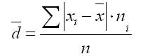
Average linear deviation is defined as the arithmetic mean of the absolute values of the deviations of individual options from .

1. For the primary row:

2. For a variation series:

where the sum of n is the sum of the frequencies of the variation series.

An example of finding the average linear deviation:

The advantage of the mean absolute deviation as a measure of dispersion over the range of variation is obvious, since this measure is based on taking into account all possible deviations. But this indicator has significant drawbacks. Arbitrary rejection of algebraic signs of deviations can lead to the fact that the mathematical properties of this indicator are far from elementary. This greatly complicates the use of the mean absolute deviation in solving problems related to probabilistic calculations.

Therefore, the average linear deviation as a measure of the variation of a feature is rarely used in statistical practice, namely when the summation of indicators without taking into account the signs makes economic sense. With its help, for example, the turnover of foreign trade, the composition of employees, the rhythm of production, etc. are analyzed.

root mean square

RMS applied, for example, to calculate the average size of the sides of n square sections, the average diameters of trunks, pipes, etc. It is divided into two types.

The root mean square is simple. If, when replacing individual values of a trait with an average value, it is necessary to keep the sum of squares of the original values unchanged, then the average will be a quadratic average.

It is the square root of the quotient of the sum of squares of individual feature values divided by their number:

The mean square weighted is calculated by the formula:

where f is a sign of weight.

Average cubic

Average cubic applied, for example, when determining the average side length and cubes. It is divided into two types.
Average cubic simple:

When calculating the mean values and dispersion in the interval distribution series, the true values of the attribute are replaced by the central values of the intervals, which are different from the arithmetic mean of the values included in the interval. This leads to a systematic error in the calculation of the variance. V.F. Sheppard determined that error in variance calculation, caused by applying the grouped data, is 1/12 of the square of the magnitude of the interval, both upward and downward in the magnitude of the variance.

Sheppard Amendment should be used if the distribution is close to normal, refers to a feature with a continuous nature of variation, built on a significant amount of initial data (n> 500). However, based on the fact that in a number of cases both errors, acting in different directions, compensate each other, it is sometimes possible to refuse to introduce amendments.

The smaller the variance and standard deviation, the more homogeneous the population and the more typical the average will be.
In the practice of statistics, it often becomes necessary to compare variations of various features. For example, it is of great interest to compare variations in the age of workers and their qualifications, length of service and wages, cost and profit, length of service and labor productivity, etc. For such comparisons, indicators of the absolute variability of characteristics are unsuitable: it is impossible to compare the variability of work experience, expressed in years, with the variation of wages, expressed in rubles.

To carry out such comparisons, as well as comparisons of the fluctuation of the same attribute in several populations with different arithmetic mean, a relative indicator of variation is used - the coefficient of variation.

Structural averages

To characterize the central trend in statistical distributions, it is often rational to use, together with the arithmetic mean, a certain value of the attribute X, which, due to certain features of its location in the distribution series, can characterize its level.

This is especially important when the extreme values of the feature in the distribution series have fuzzy boundaries. In this regard, the exact determination of the arithmetic mean, as a rule, is impossible or very difficult. In such cases, the average level can be determined by taking, for example, the value of the feature that is located in the middle of the frequency series or that occurs most often in the current series.

Such values depend only on the nature of the frequencies, i.e., on the structure of the distribution. They are typical in terms of location in the frequency series, therefore such values are considered as characteristics of the distribution center and therefore have been defined as structural averages. They are used to study the internal structure and structure of the series of distribution of attribute values. These indicators include .

Standard deviation is a classic indicator of variability from descriptive statistics.

Standard deviation, standard deviation, RMS, sample standard deviation (English standard deviation, STD, STDev) is a very common measure of dispersion in descriptive statistics. But, because technical analysis is akin to statistics, this indicator can (and should) be used in technical analysis to detect the degree of dispersion of the price of the analyzed instrument over time. Denoted by the Greek symbol Sigma "σ".

Thanks to Karl Gauss and Pearson for the fact that we have the opportunity to use the standard deviation.

Using standard deviation in technical analysis, we turn this "scattering index" in "volatility indicator“Keeping the meaning but changing the terms.

What is Standard Deviation

But in addition to intermediate auxiliary calculations, standard deviation is quite acceptable for self-calculation and applications in technical analysis. As noted by an active reader of our magazine burdock, “ I still don’t understand why RMS is not included in the set of standard indicators of domestic dealing centers«.

Really, standard deviation can in a classical and "pure" way measure the variability of an instrument. But unfortunately, this indicator is not so common in securities analysis.

Applying the Standard Deviation

Manually calculating the standard deviation is not very interesting. but useful for experience. The standard deviation can be expressed formula STD=√[(∑(x-x ) 2)/n] , which sounds like the root sum of the squared differences between the sample items and the mean, divided by the number of items in the sample.

If the number of elements in the sample exceeds 30, then the denominator of the fraction under the root takes on the value n-1. Otherwise, n is used.

step by step standard deviation calculation:

calculate the arithmetic mean of the data sample
subtract this average from each element of the sample
all the resulting differences are squared
sum all the resulting squares
divide the resulting sum by the number of elements in the sample (or by n-1 if n>30)
calculate the square root of the resulting quotient (called dispersion)

To calculate the geometric mean simple, the formula is used:

geometric weighted

To determine the geometric weighted average, the formula is used:

The average diameters of wheels, pipes, the average sides of the squares are determined using the root mean square.

RMS values are used to calculate some indicators, such as the coefficient of variation, which characterizes the rhythm of output. Here, the standard deviation from the planned output for a certain period is determined by the following formula:

These values accurately characterize the change in economic indicators compared to their base value, taken in its average value.

Quadratic simple

The mean square simple is calculated by the formula:

Quadratic weighted

The weighted root mean square is:

22. Absolute measures of variation include:

range of variation

mean linear deviation

dispersion

standard deviation

Range of variation (r)

Span variation is the difference between the maximum and minimum values of the attribute

It shows the limits in which the value of the attribute changes in the studied population.

The work experience of five applicants in the previous job is: 2,3,4,7 and 9 years. Solution: range of variation = 9 - 2 = 7 years.

For a generalized characteristic of the differences in the values of the attribute, the average variation indicators are calculated based on the allowance for deviations from the arithmetic mean. The difference is taken as the deviation from the mean.

At the same time, in order to avoid turning into zero the sum of deviations of the trait options from the mean (the zero property of the mean), one has to either ignore the signs of the deviation, that is, take this sum modulo , or square the deviation values

Mean linear and square deviation

Average linear deviation is the arithmetic mean of the absolute deviations of the individual values of the attribute from the mean.

The average linear deviation is simple:

The work experience of five applicants in the previous job is: 2,3,4,7 and 9 years.

In our example: years;

Answer: 2.4 years.

Average linear deviation weighted applies to grouped data:

The average linear deviation, due to its conditionality, is used relatively rarely in practice (in particular, to characterize the fulfillment of contractual obligations in terms of the uniformity of delivery; in the analysis of product quality, taking into account the technological features of production).

Standard deviation

The most perfect characteristic of variation is the standard deviation, which is called the standard (or standard deviation). Standard deviation() is equal to the square root of the mean square of the deviations of the individual values of the attribute from the arithmetic mean:

The standard deviation is simple:

The weighted standard deviation is applied for grouped data:

Between the mean square and mean linear deviations under conditions of normal distribution, the following relationship takes place: ~ 1.25.

When statistical testing of hypotheses, when measuring a linear relationship between random variables.

Standard deviation:

Standard deviation(an estimate of the standard deviation of the random variable Floor, walls around us and the ceiling, x relative to its mathematical expectation based on an unbiased estimate of its variance):

where - variance; - The floor, the walls around us and the ceiling, i-th sample element; - sample size; - arithmetic mean of the sample:

It should be noted that both estimates are biased. In the general case, it is impossible to construct an unbiased estimate. However, an estimate based on an unbiased variance estimate is consistent.

three sigma rule

three sigma rule() - almost all values of a normally distributed random variable lie in the interval . More strictly - with no less than 99.7% certainty, the value of a normally distributed random variable lies in the specified interval (provided that the value is true, and not obtained as a result of sample processing).

If the true value is unknown, then you should use not, but the floor, the walls around us and the ceiling, s. Thus, the rule of three sigma is translated into the rule of three Floor, walls around us and the ceiling, s .

Interpretation of the value of the standard deviation

A large value of the standard deviation shows a large spread of values in the presented set with the average value of the set; a small value, respectively, indicates that the values in the set are grouped around the average value.

For example, we have three number sets: (0, 0, 14, 14), (0, 6, 8, 14) and (6, 6, 8, 8). All three sets have mean values of 7 and standard deviations of 7, 5, and 1, respectively. The last set has a small standard deviation because the values in the set are clustered around the mean; the first set has the largest value of the standard deviation - the values within the set strongly diverge from the average value.

In a general sense, the standard deviation can be considered a measure of uncertainty. For example, in physics, the standard deviation is used to determine the error of a series of successive measurements of some quantity. This value is very important for determining the plausibility of the phenomenon under study in comparison with the value predicted by the theory: if the mean value of the measurements differs greatly from the values predicted by the theory (large standard deviation), then the obtained values or the method of obtaining them should be rechecked.

Practical use

In practice, the standard deviation allows you to determine how much the values in the set can differ from the average value.

Climate

Suppose there are two cities with the same average daily maximum temperature, but one is located on the coast and the other is inland. Coastal cities are known to have many different daily maximum temperatures less than inland cities. Therefore, the standard deviation of the maximum daily temperatures in the coastal city will be less than in the second city, despite the fact that the average value of this value is the same for them, which in practice means that the probability that the maximum air temperature of each particular day of the year will be stronger differ from the average value, higher for a city located inside the continent.

Sport

Let's assume that there are several football teams that are ranked according to some set of parameters, for example, the number of goals scored and conceded, chances to score, etc. It is most likely that the best team in this group will have the best values in more parameters. The smaller the team's standard deviation for each of the presented parameters, the more predictable the team's result is, such teams are balanced. On the other hand, a team with a large standard deviation is difficult to predict the result, which in turn is explained by an imbalance, for example, a strong defense, but a weak attack.

The use of the standard deviation of the parameters of the team allows one to predict the result of the match between two teams to some extent, evaluating the strengths and weaknesses of the teams, and hence the chosen methods of struggle.

Technical analysis

Literature

This article is proposed for deletion.

An explanation of the reasons and a corresponding discussion can be found on the page Wikipedia:To be deleted/December 17, 2012.
Until the discussion process is completed, the article can be improved, but renaming or deleting content should be refrained from, see the guide to further action for more details.
Do not remove the flag for deletion until the end of the discussion. Administrators: links here, history (last modified), logs, delete.

* Borovikov, V. STATISTICS. The art of computer data analysis: For professionals / V. Borovikov. - St. Petersburg. : Peter, 2003. - 688 p. - ISBN 5-272-00078-1.

Statistical indicators

descriptive
statistics

Continuous
data

Shear factor	Mean (Arithmetic , Geometric , Harmonic) Median Mode Range
Variation	Rank · standard deviation Coefficient of variation Quantile (Decil, Percentile/Percentile/Centile)
Moments	Mathematical expectation Dispersion Skewness Kurtosis

Discrete
data

Frequency Contingency table

Statistical
withdrawal and
examination
hypotheses

Statistical conclusion	Confidence interval (Frequency probability) Confidence interval (Bayesian inference) Statistical significance Meta-analysis
Planning experiment	Population · Sample design · Regioned sampling · Replication · Grouping · Sensitivity and specificity
Sample size	Statistical power Measure of effect Standard error
Overall score	Bayesian evaluation of a solution ·