theoretical material.

As you know, an implicitly given function of one variable is defined as follows: a function of an independent variable x is called implicit if it is given by an equation that is not resolved with respect to y:

Example 1.11.

The equation

implicitly defines two functions:

And the equation

does not define any function.

Theorem 1.2 (existence of an implicit function).

Let the function z \u003d f (x, y) and its partial derivatives f "x and f" y be defined and continuous in some neighborhood UM0 of the point M0 (x0y0). In addition, f(x0,y0)=0 and f"(x0,y0)≠0, then Eq. (1.33) defines in a neighborhood of UM0 an implicit function y= y(x), which is continuous and differentiable in some interval D centered at point x0, and y(x0)=y0.

Without proof.

From Theorem 1.2 it follows that on this interval D:

that is, there is an identity in

where the "total" derivative is found according to (1.31)

That is, (1.35) gives a formula for finding the derivative of an implicitly given function of one variable x .

An implicit function of two or more variables is defined similarly.

For example, if in some region V of the space Oxyz the following equation is true:

then under certain conditions on the function F it implicitly defines the function

At the same time, by analogy with (1.35), its partial derivatives are found as follows:

Example 1.12. Assuming that the equation

implicitly defines a function

find z "x, z" y.

therefore, according to (1.37), we obtain the answer.

11. Use of partial derivatives in geometry.

12. Extrema of a function of two variables.

The concepts of maximum, minimum, extremum of a function of two variables are similar to the corresponding concepts of a function of one independent variable (see Section 25.4).

Let the function z = ƒ(х;у) be defined in some domain D, the point N(x0;y0) н D.

A point (x0; y0) is called a maximum point of the function z=ƒ(x; y) if there is such a d-neighbourhood of the point (x0; y0) that for each point (x; y) other than (xo; yo), this neighborhood satisfies the inequality ƒ(х;у)<ƒ(хо;уо).

BUT the minimum point of the function is defined logically: for all points (x; y) other than (x0; y0), the following inequality holds from the d-neighborhood of the point (xo; yo): ƒ(x; y)>ƒ(x0; y0).

In Figure 210: N1 is the maximum point, and N2 is the minimum point of the function z=ƒ(x;y).

The value of the function at the point of maximum (minimum) is called the maximum (minimum) of the function. The maximum and minimum of a function are called its extrema.

Note that, by virtue of the definition, the extremum point of the function lies inside the domain of the function; the maximum and minimum have a local (local) character: the value of the function at the point (x0; y0) is compared with its values ​​at points sufficiently close to (x0; y0). In region D, the function may have several extrema or none.

46.2. Necessary and sufficient conditions for an extremum

Consider the conditions for the existence of an extremum of a function.

Theorem 46.1 (necessary conditions for an extremum). If at the point N (x0; y0) the differentiable function z \u003d ƒ (x; y) has an extremum, then its partial derivatives at this point are equal to zero: ƒ "x (x0; y0) \u003d 0, ƒ" y (x0; y0 )=0.

We fix one of the variables. Suppose, for example, y=y0. Then we get the function ƒ(x; y0)=φ(x) of one variable, which has an extremum at x = x0. Therefore, according to the necessary condition for the extremum of a function of one variable (see paragraph 25.4), φ "(x0) \u003d 0, that is, ƒ "x (x0; y0) \u003d 0.

Similarly, it can be shown that ƒ "y (x0; y0) \u003d 0.

Geometrically, the equalities ƒ "x (x0; y0) \u003d 0 and ƒ "y (x0; y0) \u003d 0 mean that at the extremum point of the function z \u003d ƒ (x; y), the tangent plane to the surface depicting the function ƒ (x; y ), is parallel to the Oxy plane, since the equation of the tangent plane is z=z0 (see formula (45.2)).

W note. A function can have an extremum at points where at least one of the partial derivatives does not exist. For example, the function has a maximum at the point O (0; 0) (see Fig. 211), but has no partial derivatives at this point.

The point at which the first order partial derivatives of the function z ≈ ƒ(x; y) are equal to zero, i.e. f "x=0, f" y=0, is called the stationary point of the function z.

Stationary points and points where at least one partial derivative does not exist are called critical points.

At critical points, the function may or may not have an extremum. Equality to zero of partial derivatives is a necessary but not sufficient condition for the existence of an extremum. Consider, for example, the function z = xy. For her, the point O (0; 0) is critical (in it z "x \u003d y and z" y - x vanish). However, the function z=xy does not have an extremum in it, since in a sufficiently small neighborhood of the point O(0; 0) there are points for which z>0 (points I and III of quarters) and z< 0 (точки II и IV четвертей).

Thus, in order to find the extrema of the function in a given region, it is necessary to subject each critical point of the function to an additional study.

Theorem 46.2 (sufficient condition for an extremum). Let the function ƒ(x; y) have continuous partial derivatives up to the second order inclusive at a stationary point (xo; yo) and some of its neighborhood. Let us calculate at the point (x0;y0) the values ​​A=f""xx(x0;y0), B=ƒ""xy(x0;y0), C=ƒ""yy(x0;y0). Denote

1. if Δ > 0, then the function ƒ(x; y) at the point (x0; y0) has an extremum: maximum if A< 0; минимум, если А > 0;

2. if Δ< 0, то функция ƒ(х;у) в точке (х0;у0) экстремума не имеет.

In the case of Δ = 0, there may or may not be an extremum at the point (x0; y0). More research is needed.

TASKS

1.

Example. Find the intervals of increase and decrease of the function . Decision. The first step is finding the area of ​​function definitions. In our example, the expression in the denominator should not vanish, therefore, . Let's move on to the derivative function: To determine the intervals of increase and decrease of a function by a sufficient criterion, we solve the inequalities and on the domain of definition. Let us use a generalization of the interval method. The only real root of the numerator is x=2, and the denominator vanishes at x=0. These points divide the domain of definition into intervals in which the derivative of the function retains its sign. Let's mark these points on the number line. By pluses and minuses, we conditionally denote the intervals on which the derivative is positive or negative. The arrows below schematically show the increase or decrease of the function on the corresponding interval. Thus, and . At the point x=2 the function is defined and continuous, so it must be added to both the increasing interval and the decreasing interval. At the point x=0 the function is not defined, so this point is not included in the required intervals. We present the graph of the function to compare the obtained results with it. Answer: the function increases with , decreases on the interval (0; 2] .

2.

Examples.

Set intervals for convexity and concavity of a curve y = 2 – x 2 .

Let's find y"" and determine where the second derivative is positive and where it is negative. y" = –2x, y"" = –2 < 0 на (–∞; +∞), следовательно, функция всюду выпукла.

y = e x. As y"" = e x > 0 for any x, then the curve is concave everywhere.

y = x 3 . As y"" = 6x, then y"" < 0 при x < 0 и y"" > 0 when x> 0. Therefore, at x < 0 кривая выпукла, а при x> 0 is concave.

3.

4. Given a function z=x^2-y^2+5x+4y, a vector l=3i-4j and a point A(3,2). Find dz/dl (as I understand it, the derivative of the function in the direction of the vector), gradz(A), |gradz(A)|. Find partial derivatives: z(in x)=2x+5 z(in y)=-2y+4 Find the values ​​of derivatives at point A(3,2): z(in x)(3,2)=2*3+ 5=11 z(by y)(3,2)=-2*2+4=0 ^2)=11 Derivative of the function z in the direction of the vector l: dz/dl=z(in x)*cosa+z(in y)*cosb, a,b-angles of the vector l with the coordinate axes. cosa=lх/|l|, cosb=ly/|l|, |l|=sqrt(lx^2+ly^2) lx=3, ly=-4, |l|=5. cosa=3/5, cosb=(-4)/5. dz/dl=11*3/5+0*(-4)/5=6.6.

Let the function be given implicitly using the equation
(1) .
And let this equation, for some value , has a unique solution . Let the function be a differentiable function at the point , and
.
Then, for this value , there is a derivative , which is determined by the formula:
(2) .

Proof

For proof, consider the function as a complex function of the variable :
.
We apply the rule of differentiation of a complex function and find the derivative with respect to the variable of the left and right sides of the equation
(3) :
.
Since the derivative of the constant is equal to zero and , then
(4) ;
.

The formula has been proven.

Derivatives of higher orders

Let us rewrite equation (4) using other notation:
(4) .
Moreover, and are complex functions of the variable :
;
.
Dependence defines the equation (1):
(1) .

We find the derivative with respect to the variable from the left and right sides of equation (4).
According to the formula for the derivative of a complex function, we have:
;
.
According to the derivative product formula:

.
According to the derivative sum formula:


.

Since the derivative of the right side of equation (4) is equal to zero, then
(5) .
Substituting the derivative here, we obtain the value of the second-order derivative in implicit form.

Differentiating equation (5) in a similar way, we obtain an equation containing a third order derivative:
.
Substituting here the found values ​​of the derivatives of the first and second orders, we find the value of the third order derivative.

Continuing differentiation, one can find a derivative of any order.

Examples

Example 1

Find the first derivative of the function given implicitly by the equation:
(P1) .

Formula 2 Solution

We find the derivative by formula (2):
(2) .

Let's move all the variables to the left side so that the equation takes the form .
.
From here.

We find the derivative with respect to , assuming that it is constant.
;
;
;
.

We find the derivative with respect to the variable, assuming the variable is constant.
;
;
;
.

By formula (2) we find:
.

We can simplify the result if we note that according to the original equation (A.1), . Substitute :
.
Multiply the numerator and denominator by:
.

Solution in the second way

Let's solve this example in the second way. To do this, we find the derivative with respect to the variable of the left and right parts of the original equation (P1).

We apply:
.
We apply the formula for the derivative of a fraction:
;
.
We apply the formula for the derivative of a complex function:
.
We differentiate the original equation (P1).
(P1) ;
;
.
Multiply by and group the terms.
;
.

Substitute (from equation (P1)):
.
Let's multiply by:
.

Answer

Example 2

Find the second order derivative of the function given implicitly using the equation:
(P2.1) .

Decision

Differentiate the original equation with respect to the variable , assuming that it is a function of :
;
.
We apply the formula for the derivative of a complex function.
.

We differentiate the original equation (A2.1):
;
.
It follows from the original equation (A2.1) that . Substitute :
.
Expand the brackets and group the members:
;
(P2.2) .
We find the derivative of the first order:
(P2.3) .

To find the second order derivative, we differentiate equation (A2.2).
;
;
;
.
We substitute the expression for the first order derivative (A2.3):
.
Let's multiply by:

;
.
From here we find the derivative of the second order.

Answer

Example 3

Find the third order derivative for of the function given implicitly using the equation:
(P3.1) .

Decision

Differentiate the original equation with respect to the variable, assuming that is a function of .
;
;
;
;
;
;
(P3.2) ;

We differentiate equation (A3.2) with respect to the variable .
;
;
;
;
;
(P3.3) .

We differentiate equation (A3.3).
;
;
;
;
;
(P3.4) .

From equations (A3.2), (A3.3) and (A3.4) we find the values ​​of derivatives at .
;
;
.

We will learn to find derivatives of functions that are given implicitly, that is, given by some equations that relate variables to each other x and y. Examples of functions defined implicitly:

,

,

Derivatives of implicit functions, or derivatives of implicit functions, are fairly easy to find. Now let's analyze the corresponding rule and example, and then find out why this is needed at all.

In order to find the derivative of a function given implicitly, it is necessary to differentiate both sides of the equation with respect to x. Those terms in which only x is present will turn into the usual derivative of a function of x. And the terms with y must be differentiated using the rule of differentiation of a complex function, since y is a function of x. If it’s quite simple, then in the resulting derivative of the term with x it should turn out: the derivative of the function from the y, multiplied by the derivative from the y. For example, the derivative of the term will be written as , the derivative of the term will be written as . Further, from all this it is necessary to express this "y stroke" and the desired derivative of the function given implicitly will be obtained. Let's look at this with an example.

Example 1

Decision. We differentiate both sides of the equation with respect to x, assuming that y is a function of x:

From here we get the derivative that is required in the task:

Now something about the ambiguous property of implicitly defined functions, and why special rules for their differentiation are needed. In some cases, you can make sure that substitution in a given equation (see examples above) instead of the y of its expression through x leads to the fact that this equation turns into an identity. So. the above equation implicitly defines the following functions:

After substituting the expression y squared through x into the original equation, we get the identity:

.

The expressions that we substituted were obtained by solving the equation for the y.

If we were to differentiate the corresponding explicit function

then we would get a response as in example 1 - from a function specified implicitly:

But not every function given implicitly can be represented in the form y = f(x) . So, for example, the implicitly defined functions

are not expressed in terms of elementary functions, that is, these equations cannot be solved with respect to the player. Therefore, there is a rule for differentiating a function given implicitly, which we have already studied and will be consistently applied in other examples.

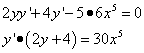
Example 2 Find the derivative of a function given implicitly:

.

We express the y prime and - at the output - the derivative of the function given implicitly:

Example 3 Find the derivative of a function given implicitly:

.

Decision. Differentiate both sides of the equation with respect to x:

.

Example 4 Find the derivative of a function given implicitly:

.

Decision. Differentiate both sides of the equation with respect to x:

.

We express and get the derivative:

.

Example 5 Find the derivative of a function given implicitly:

Decision. We transfer the terms on the right side of the equation to the left side and leave zero on the right. Differentiate both sides of the equation with respect to x.

Given a system of equations

or brieflyF(x, y)=0 (1)

Definition. System (1) defines an implicitly defined functiony= f(x) on theD R n

,

if x D : F(x , f(x)) = 0.

Theorem (existence and uniqueness of a mapping implicitly defined by a system of equations). Let be

Then in some neighborhoodU (x 0 ) there is a unique function (mapping) defined in this neighborhoody = f(x), such that

 x U (x 0 ) : F(x, f(x))=0 andy 0 = f(x 0 ).

This function is continuously differentiable in some neighborhood of the pointx 0 .

5. Calculation of derivatives of implicit functions given by a system of equations

Given system

(1)

We will assume that the conditions of the existence and uniqueness theorem for the implicit function given by this system of equations are satisfied. We denote this function y= f(x) . Then in some neighborhood of the point x 0 the identities

(F(x, f(x))=0) (2)

Differentiating these identities with respect to x j we get

=0 (3)

These equalities can be written in matrix form

, (3)

or expanded

.

Note that the transition from equality F(x, f(x))=0 to
, corresponds to the rules of differentiation for the case when x and y are points in one-dimensional space. Matrix is not degenerate by assumption, so the matrix equation
has a solution
. Thus, one can find first-order partial derivatives of implicit functions . To find the differentials, we denote

dy = ,dx = , differentiating the equalities (2) we get

=0 ,

or in matrix form

. (4)

Expanded

.

As in the case of partial derivatives, the formula (4) we have the same form as for the case of one-dimensional spaces n=1, p=1. The solution to this matrix equation can be written as
. To find partial derivatives of the second order, it will be necessary to differentiate the identities (3) (to calculate second-order differentials, you need to differentiate the identities (4) ). Thus, we get

,

where through A the terms that do not contain the desired ones are indicated
.

The matrix of coefficients of this system for determining derivatives
is the Jacobian matrix .

A similar formula can be obtained for differentials. In each of these cases, a matrix equation will be obtained with the same matrix of coefficients in a system of equations to determine the desired derivatives or differentials. The same will happen under the following differentiations.

Example 1. Find ,,at the point u=1, v=1.

Decision. Differentiate the given equalities

(5)

Note that, according to the formulation of the problem, we should consider as independent variables x, y. Then the functions will be z, u, v. Thus the system (5) to decide on the unknown du, dv, dz . In matrix form, it looks like this

.

Let's solve this system using Cramer's rule. Coefficient matrix determinant

, The third "replaced" determinant for dz will be equal to (it is calculated by expanding on the last column)

, then

dz =
, and
,
.

Differentiating (5) again ( x, y – independent variables)

The coefficient matrix of the system is the same, the third determinant

Solving this system, we obtain an expression for d 2 z where you can find the desired derivative.

Implicit functions defined by a system of equations

Given a system of equations

or briefly F(x,y)= 0. (6.7)

Definition. System(6.7)defines an implicit function y=f(x)to DÌR n

if "xОD:F(x , f(x)) = 0.

Theorem (existence and uniqueness of a mapping implicitly defined by a system of equations).Let be

1) F i(x,y)from (6.4) are defined and have continuous partial derivatives of the first order, (i= 1,…,p, k= 1,…,n, j= 1,…,p) in the neighborhood U(M 0)points M 0 (x 0 ,y 0), x 0 = , y 0 =

2) F(M 0)=0,

3) det.

Then in some neighborhood U(x 0)there is a unique function (mapping) defined in this neighborhood y = f(x), such that

"xО U(x 0) :F(x, f(x))=0and y 0 = f(x 0).

This function is continuously differentiable in some neighborhood of the point x 0 .

Given system

We will assume that the conditions of the existence and uniqueness theorem for the implicit function given by this system of equations are satisfied. We denote this function y=f(x) . Then in some neighborhood of the point x 0 the identities are valid

Differentiating these identities with respect to xj we get

= 0.(6.9)

These equalities can be written in matrix form

or expanded

Note that the transition from equality F(x, f(x))=0k , corresponds to the rules of differentiation for the case when x and y are points in one-dimensional space. The matrix is ​​not degenerate by condition, so the matrix equation has a solution. Thus, it is possible to find first-order partial derivatives of implicit functions. To find the differentials, we denote

dy= , dx=, differentiating equalities (6.8), we obtain

or in matrix form

Expanded

Just as in the case of partial derivatives, formula (6.10) has the same form as in the case of one-dimensional spaces n= 1, p= 1. The solution of this matrix equation can be written as To find partial derivatives of the second order, it will be necessary to differentiate identities (6.9) (to calculate second-order differentials, it is necessary to differentiate identities (6.10)). Thus, we get

where through A the terms that do not contain the desired ones are denoted.

The coefficient matrix of this system for determining the derivatives is the Jacobi matrix.

A similar formula can be obtained for differentials. In each of these cases, a matrix equation will be obtained with the same matrix of coefficients in the system of equations for determining the desired derivatives or differentials. The same will happen under the following differentiations.

Example 1 Find, at a point u= 1,v= 1.

Decision. Differentiate the given equalities

Note that it follows from the condition of the problem that we should consider as independent variables x, y. Then the functions will be z, u, v. Thus, the system (6.11) should be solved with respect to the unknowns du, dv, dz. In matrix form, it looks like this

Let's solve this system using Cramer's rule. Coefficient matrix determinant

The third "replaced" determinant for dz will be equal to (it is calculated by expanding on the last column)

dz = , and, .

We differentiate (6.11) again ( x, y- independent variables)

The coefficient matrix of the system is the same, the third determinant

Solving this system, we obtain an expression for d2z where you can find the desired derivative.

6.3. Differentiable mappings

Derivative mappings. Regular displays. Necessary and sufficient conditions for functional dependence.