Matrix norms. Consistency and subordination of norms

» Lesson 12. Matrix rank. Matrix rank calculation. Matrix norm

Lesson number 12. Matrix rank. Matrix rank calculation. Matrix norm.

If all matrix minorsAorderkare equal to zero, then all minors of order k + 1, if such exist, are also equal to zero.
Matrix rank A is the largest order of the minors of the matrix A , other than zero.
The maximum rank can be equal to the minimum number of the number of rows or columns of the matrix, i.e. if the matrix has a size of 4x5, then the maximum rank will be 4.
The minimum rank of a matrix is 1, unless you are dealing with a zero matrix, where the rank is always zero.

The rank of a nondegenerate square matrix of order n is equal to n, since its determinant is a minor of order n and the nondegenerate matrix is nonzero.
Transposing a matrix does not change its rank.

Let the rank of the matrix be . Then any minor of order , other than zero, is called basic minor.
Example. Given a matrix A.

The matrix determinant is zero.
Minor of the second order . Therefore, r(A)=2 and the minor is basic.
A basic minor is also a minor .
Minor , because =0, so it will not be basic.
Exercise: independently check which other second-order minors will be basic and which will not.

Finding the rank of a matrix by calculating all its minors requires too much computational work. (The reader can verify that there are 36 second-order minors in a fourth-order square matrix.) Therefore, a different algorithm is used to find the rank. To describe it, some additional information is required.

We call the following operations on them elementary transformations of matrices:
1) permutation of rows or columns;
2) multiplying a row or column by a non-zero number;
3) adding to one of the rows another row, multiplied by a number, or adding to one of the columns of another column, multiplied by a number.

Under elementary transformations, the rank of the matrix does not change.
Algorithm for calculating the rank of a matrix is similar to the determinant calculation algorithm and lies in the fact that with the help of elementary transformations the matrix is reduced to a simple form for which it is not difficult to find the rank. Since the rank did not change with each transformation, by calculating the rank of the transformed matrix, we thereby find the rank of the original matrix.

Let it be required to calculate the rank of the matrix of dimensions mxn.

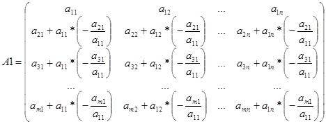
As a result of calculations, the matrix A1 has the form

If all rows, starting from the third one, are zero, then , since minor . Otherwise, by permuting rows and columns with numbers greater than two, we achieve that the third element of the third row is different from zero. Further, by adding the third row, multiplied by the corresponding numbers, to the rows with large numbers, we get zeros in the third column, starting from the fourth element, and so on.
At some stage, we will come to a matrix in which all rows, starting from (r + 1) th, are equal to zero (or absent at ), and the minor in the first rows and first columns is the determinant of a triangular matrix with non-zero elements on the diagonal . The rank of such a matrix is . Therefore, Rang(A)=r.

In the proposed algorithm for finding the rank of a matrix, all calculations must be performed without rounding. An arbitrarily small change in at least one of the elements of the intermediate matrices can lead to the fact that the resulting answer will differ from the rank of the original matrix by several units.
If the elements in the original matrix were integers, then it is convenient to perform calculations without using fractions. Therefore, at each stage, it is advisable to multiply the strings by such numbers that no fractions appear in the calculations.

In laboratory and practical work, we will consider an example of finding the rank of a matrix.

FINDING ALGORITHM MATRIX REGULATIONS .
There are only three norms of the matrix.
First Matrix Norm= the maximum of the numbers obtained by adding all the elements of each column, taken modulo.
Example: let a 3x2 matrix A be given (Fig. 10). The first column contains elements: 8, 3, 8. All elements are positive. Let's find their sum: 8+3+8=19. The second column contains the elements: 8, -2, -8. Two elements are negative, therefore, when adding these numbers, it is necessary to substitute the modulus of these numbers (that is, without the minus signs). Let's find their sum: 8+2+8=18. The maximum of these two numbers is 19. So the first norm of the matrix is \u200b\u200b19.

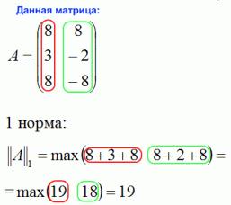
Figure 10.

Second Matrix Norm is the square root of the sum of the squares of all matrix elements. And this means we square all the elements of the matrix, then add the resulting values \u200b\u200band extract the square root from the result.
In our case, the 2 norm of the matrix turned out to be equal to the square root of 269. In the diagram, I roughly took the square root of 269 and the result was approximately 16.401. Although it is more correct not to extract the root.

Third Norm Matrix is the maximum of the numbers obtained by adding all the elements of each row, taken modulo.
In our example: the first line contains elements: 8, 8. All elements are positive. Let's find their sum: 8+8=16. The second line contains elements: 3, -2. One of the elements is negative, so when adding these numbers, you must substitute the modulus of this number. Let's find their sum: 3+2=5. The third line contains the elements 8, and -8. One of the elements is negative, so when adding these numbers, you must substitute the modulus of this number. Let's find their sum: 8+8=16. The maximum of these three numbers is 16. So the third norm of the matrix is \u200b\u200b16.

Compiled by: Saliy N.A.

Matrix norm we call the real number assigned to this matrix ||A|| such that, as a real number, it is assigned to each matrix from the n-dimensional space and satisfies 4 axioms:

1. ||A||³0 and ||A||=0 only if A is a zero matrix;

2. ||αA||=|α|·||A||, where a R;

3. ||A+B||£||A||+||B||;

4. ||A·B||£||A||·||B||. (property of multiplicativity)

The matrix norm can be entered in various ways. Matrix A can be viewed as n 2 - dimensional vector.

This norm is called the Euclidean norm of a matrix.

If for any square matrix A and any vector x whose dimension is equal to the order of the matrix, the inequality ||Ax||£||A||·||x||

then we say that the norm of the matrix A is consistent with the norm of the vector. Note that the norm of the vector is on the left in the last condition (Ax is a vector).

Various matrix norms are consistent with a given vector norm. Let's choose the smallest among them. Such will be

This matrix norm is subordinate to the given vector norm. The existence of a maximum in this expression follows from the continuity of the norm, since there always exists a vector x -> ||x||=1 and ||Ax||=||A||.

Let us show that xthen the norm N(A) is not subject to any vector norm. Matrix norms subordinate to the previously introduced vector norms are expressed as follows:

1. ||A|| ¥ = |a ij | (norm-maximum)

2. ||A|| 1 = |a ij | (norm-sum)

3. ||A|| 2 = , (spectral norm)

where s 1 is the largest eigenvalue of the symmetric matrix A¢A, which is the product of the transposed and original matrices. If the matrix A¢A is symmetric, then all its eigenvalues are real and positive. The number l is an eigenvalue, and a nonzero vector x is an eigenvector of the matrix A (if they are related by the relation Ax=lx). If the matrix A is itself symmetric, A¢ = A, then A¢A = A 2 and then s 1 = , where is the eigenvalue of the matrix A with the greatest absolute value. Therefore, in this case we have = .

Matrix eigenvalues do not exceed any of its agreed norms. Normalizing the relation defining the eigenvalues, we obtain ||λx||=||Ax||, |λ|·||x||=||Ax||£||A||·||x||, |λ| £||A||

Since ||A|| 2 £||A|| e , where the Euclidean norm can be calculated simply, instead of the spectral norm, the Euclidean norm of the matrix can be used in estimates.

30. Conditionality of systems of equations. Conditioning factor .

Degree of conditionality- influence of the decision on the initial data. ax = b: vector b corresponds decision x. Let b will change by . Then the vector b+ will match the new solution x+ : A(x+ ) = b+. Since the system is linear, then Ax+A = b+, then A = ; = ; = ; b = Ax; = then ; * , where is the relative error of the perturbation of the solution, – conditioning factorcond(A) (how many times the error of the solution can increase), is the relative perturbation of the vector b. cond(A) = ; cond(A)* Coefficient properties: depends on the choice of the matrix norm; cond( = cond(A); multiplying a matrix by a number does not affect the condition factor. The larger the coefficient, the stronger the error in the initial data affects the solution of the SLAE. The condition number cannot be less than 1.

31. Sweep method for solving systems of linear algebraic equations.

Often there is a need to solve systems whose matrices, being weakly filled, i.e. containing many non-zero elements. The matrices of such systems usually have a certain structure, among which there are systems with band structure matrices, i.e. in them, nonzero elements are located on the main diagonal and on several secondary diagonals. To solve systems with band matrices, the Gaussian method can be transformed into more efficient methods. Let us consider the simplest case of tape systems, to which, as we will see later, the solution of discretization problems for boundary value problems for differential equations is reduced by the methods of finite differences, finite elements, etc. A three-diagonal matrix is such a matrix that has nonzero elements only on the main diagonal and adjacent to it:

The three diagonal matrix of non-zero elements has a total of (3n-2).

Rename the coefficients of the matrix:

Then, in component-by-component notation, the system can be represented as:

A i * x i-1 + b i * x i + c i * x i+1 = d i , i=1, 2,…, n; (7)

a 1 =0, c n =0. (eight)

The structure of the system assumes the relationship only between neighboring unknowns:

x i \u003d x i * x i +1 + h i (9)

x i -1 =x i -1* x i + h i -1 and substitute into (7):

A i (x i-1* x i + h i-1)+ b i * x i + c i * x i+1 = d i

(a i * x i-1 + b i)x i = –c i * x i+1 +d i –a i * h i-1

Comparing the resulting expression with representation (7), we obtain:

Formulas (10) represent recursive relations for calculating sweep coefficients. They require initial values to be specified. In accordance with the first condition (8) for i =1 we have a 1 =0, which means

Further, the remaining sweep coefficients are calculated and stored according to formulas (10) for i=2,3,…, n, and for i=n, taking into account the second condition (8), we obtain x n =0. Therefore, in accordance with formula (9) x n = h n .

After that, according to the formula (9), the unknowns x n -1 , x n -2 , …, x 1 are sequentially found. This stage of the calculation is called the reverse run, while the calculation of the sweep coefficients is called the forward sweep.

For the successful application of the sweep method, it is necessary that in the process of calculations there are no situations with division by zero, and with a large dimensionality of the systems there should not be a rapid increase in rounding errors. We will call the run correct, if the denominator of the sweep coefficients (10) does not vanish, and sustainable, if ½x i ½<1 при всех i=1,2,…, n. Достаточные условия корректности и устойчивости прогонки, которые во многих приложениях выполняются, определяются теоремой.

Theorem. Let coefficients a i and c i of equation (7) for i=2,3,..., n-1 be different from zero and let

½b i ½>½a i ½+½c i ½ for i=1, 2,..., n. (eleven)

Then the sweep defined by formulas (10), (9) is correct and stable.

Encyclopedic YouTube

1 / 1

✪ Vector norm. Part 4

Subtitles

Definition

Let K be the main field (usually K = R or K = C ) and is the linear space of all matrices with m rows and n columns, consisting of elements of K . A norm is given on the space of matrices if each matrix is associated with a non-negative real number ‖ A ‖ (\displaystyle \|A\|), called its norm, so that

In the case of square matrices (i.e. m = n), matrices can be multiplied without leaving the space, and therefore the norms in these spaces usually also satisfy the property submultiplicativity :

Submultiplicativity can also be performed for the norms of non-square matrices, but defined for several required sizes at once. Namely, if A is a matrix ℓ × m, and B is the matrix m × n, then A B- matrix ℓ × n .

Operator norms

An important class of matrix norms are operator norms, also referred to as subordinates or induced . The operator norm is uniquely constructed according to the two norms defined in and , based on the fact that any matrix m × n is represented by a linear operator from K n (\displaystyle K^(n)) in K m (\displaystyle K^(m)). Specifically,

‖ A ‖ = sup ( ‖ A x ‖ : x ∈ K n , ‖ x ‖ = 1 ) = sup ( ‖ A x ‖ ‖ x ‖ : x ∈ K n , x ≠ 0 ) . (\displaystyle (\begin(aligned)\|A\|&=\sup\(\|Ax\|:x\in K^(n),\ \|x\|=1\)\\&=\ sup \left\((\frac (\|Ax\|)(\|x\|)):x\in K^(n),\ x\neq 0\right\).\end(aligned)))

Under the condition that norms on vector spaces are consistently specified, such a norm is submultiplicative (see ).

Examples of operator norms

Properties of the spectral norm:

The spectral norm of an operator is equal to the maximum singular value of this operator.
The spectral norm of a normal operator is equal to the absolute value of the maximum modulo eigenvalue of this operator.
The spectral norm does not change when a matrix is multiplied by an orthogonal (unitary) matrix.

Non-operator norms of matrices

There are matrix norms that are not operator norms. The concept of non-operator norms of matrices was introduced by Yu. I. Lyubich and studied by G. R. Belitsky.

An example of a non-operator norm

For example, consider two different operator norms ‖ A ‖ 1 (\displaystyle \|A\|_(1)) and ‖ A ‖ 2 (\displaystyle \|A\|_(2)), such as row and column norms. Forming a new norm ‖ A ‖ = m a x (‖ A ‖ 1 , ‖ A ‖ 2) (\displaystyle \|A\|=max(\|A\|_(1),\|A\|_(2))). The new norm has an annular property ‖ A B ‖ ≤ ‖ A ‖ ‖ B ‖ (\displaystyle \|AB\|\leq \|A\|\|B\|), preserves the unit ‖ I ‖ = 1 (\displaystyle \|I\|=1) and is not operator .

Examples of norms

Vector p (\displaystyle p)-norm

Can be considered m × n (\displaystyle m\times n) matrix as a size vector m n (\displaystyle mn) and use standard vector norms:

‖ A ‖ p = ‖ v e c (A) ‖ p = (∑ i = 1 m ∑ j = 1 n | a i j | p) 1 / p (\displaystyle \|A\|_(p)=\|\mathrm ( vec) (A)\|_(p)=\left(\sum _(i=1)^(m)\sum _(j=1)^(n)|a_(ij)|^(p)\ right)^(1/p))

Frobenius norm

Frobenius norm, or euclidean norm is a special case of the p-norm for p = 2 : ‖ A ‖ F = ∑ i = 1 m ∑ j = 1 n a i j 2 (\displaystyle \|A\|_(F)=(\sqrt (\sum _(i=1)^(m)\sum _(j =1)^(n)a_(ij)^(2)))).

The Frobenius norm is easy to calculate (compared to, for example, the spectral norm). It has the following properties:

‖ A x ‖ 2 2 = ∑ i = 1 m | ∑ j = 1 n a i j x j | 2 ≤ ∑ i = 1 m (∑ j = 1 n | a i j | 2 ∑ j = 1 n | x j | 2) = ∑ j = 1 n | x j | 2 ‖ A ‖ F 2 = ‖ A ‖ F 2 ‖ x ‖ 2 2 . (\displaystyle \|Ax\|_(2)^(2)=\sum _(i=1)^(m)\left|\sum _(j=1)^(n)a_(ij)x_( j)\right|^(2)\leq \sum _(i=1)^(m)\left(\sum _(j=1)^(n)|a_(ij)|^(2)\sum _(j=1)^(n)|x_(j)|^(2)\right)=\sum _(j=1)^(n)|x_(j)|^(2)\|A\ |_(F)^(2)=\|A\|_(F)^(2)\|x\|_(2)^(2).)

Submultiplicativity: ‖ A B ‖ F ≤ ‖ A ‖ F ‖ B ‖ F (\displaystyle \|AB\|_(F)\leq \|A\|_(F)\|B\|_(F)), because ‖ A B ‖ F 2 = ∑ i , j | ∑ k a i k b k j | 2 ≤ ∑ i , j (∑ k | a i k | | b k j |) 2 ≤ ∑ i , j (∑ k | a i k | 2 ∑ k | b k j | 2) = ∑ i , k | a i k | 2 ∑ k , j | b k j | 2 = ‖ A ‖ F 2 ‖ B ‖ F 2 (\displaystyle \|AB\|_(F)^(2)=\sum _(i,j)\left|\sum _(k)a_(ik) b_(kj)\right|^(2)\leq \sum _(i,j)\left(\sum _(k)|a_(ik)||b_(kj)|\right)^(2)\ leq \sum _(i,j)\left(\sum _(k)|a_(ik)|^(2)\sum _(k)|b_(kj)|^(2)\right)=\sum _(i,k)|a_(ik)|^(2)\sum _(k,j)|b_(kj)|^(2)=\|A\|_(F)^(2)\| B\|_(F)^(2)).
‖ A ‖ F 2 = t r ⁡ A ∗ A = t r ⁡ A A ∗ (\displaystyle \|A\|_(F)^(2)=\mathop (\rm (tr)) A^(*)A=\ mathop (\rm (tr)) AA^(*)), where t r ⁡ A (\displaystyle \mathop (\rm (tr)) A)- matrix trace A (\displaystyle A), A ∗ (\displaystyle A^(*)) is a Hermitian conjugate matrix .
‖ A ‖ F 2 = ρ 1 2 + ρ 2 2 + ⋯ + ρ n 2 (\displaystyle \|A\|_(F)^(2)=\rho _(1)^(2)+\rho _ (2)^(2)+\dots +\rho _(n)^(2)), where ρ 1 , ρ 2 , … , ρ n (\displaystyle \rho _(1),\rho _(2),\dots ,\rho _(n))- singular values of the matrix A (\displaystyle A).
‖ A ‖ F (\displaystyle \|A\|_(F)) does not change when multiplying a matrix A (\displaystyle A) left or right onto orthogonal (unitary) matrices.

Module maximum

The maximum modulus norm is another special case of the p-norm for p = ∞ .

‖ A ‖ max = max ( | a i j | ) . (\displaystyle \|A\|_(\text(max))=\max\(|a_(ij)|\).)

Norm Shatten

Consistency of matrix and vector norms

‖ A x ‖ b ≤ ‖ A ‖ a b ‖ x ‖ a (\displaystyle \|Ax\|_(b)\leq \|A\|_(ab)\|x\|_(a))

for any A ∈ K m × n , x ∈ K n (\displaystyle A\in K^(m\times n),x\in K^(n)). By construction, the operator norm is consistent with the original vector norm.

Examples of consistent but not subordinate matrix norms:

Equivalence of norms

All norms in space K m × n (\displaystyle K^(m\times n)) are equivalent, that is, for any two norms ‖ . α (\displaystyle \|.\|_(\alpha )) and ‖ . ‖ β (\displaystyle \|.\|_(\beta )) and for any matrix A ∈ K m × n (\displaystyle A\in K^(m\times n)) double inequality is true.