Relative error of the ith period. Absolute and relative measurement errors

Measurement error- assessment of the deviation of the measured value of a quantity from its true value. Measurement error is a characteristic (measure) of measurement accuracy.

Because to find out with absolute precision true value no value is possible, then it is also impossible to indicate the magnitude of the deviation of the measured value from the true value. (This deviation is usually called the measurement error. In a number of sources, for example, in the Bolshoi Soviet encyclopedia, terms measurement error and measurement error are used as synonyms, but according to RMG 29-99 the term measurement error not recommended as less successful). It is only possible to estimate the magnitude of this deviation, for example, using statistical methods. In practice, instead of the true value, we use actual value x d, that is, the value of a physical quantity obtained experimentally and so close to the true value that it can be used instead of it in the set measurement task. This value is usually calculated as the average value obtained from statistical processing results of a series of measurements. This value obtained is not exact, but only the most probable. Therefore, it is necessary to indicate in the measurements what their accuracy is. To do this, along with the result obtained, the measurement error is indicated. For example, the entry T=2.8±0.1 c. means that the true value of the quantity T lies in the interval from 2.7 s before 2.9 s with some specified probability

In 2004 on international level was accepted new document, dictating the conditions for carrying out measurements and establishing new rules for comparing state standards. The concept of "error" became obsolete, the concept of "measurement uncertainty" was introduced instead, however, GOST R 50.2.038-2004 allows the use of the term error for documents used in Russia.

There are the following types of errors:

The absolute error

Relative error

the reduced error;

The main error

Additional error

· systematic error;

Random error

Instrumental error

· methodical error;

· personal error;

· static error;

dynamic error.

Measurement errors are classified according to the following criteria.

· According to the method of mathematical expression, the errors are divided into absolute errors and relative errors.

· According to the interaction of changes in time and the input value, the errors are divided into static errors and dynamic errors.

By the nature of the occurrence of errors are divided into systematic errors and random errors.

· According to the nature of the dependence of the error on the influencing values, the errors are divided into basic and additional.

· According to the nature of the dependence of the error on the input value, the errors are divided into additive and multiplicative.

Absolute error is the value calculated as the difference between the value of the quantity obtained during the measurement process and the real (actual) value of the given quantity. The absolute error is calculated using the following formula:

AQ n =Q n /Q 0 , where AQ n is the absolute error; Qn- the value of a certain quantity obtained in the process of measurement; Q0- the value of the same quantity, taken as the base of comparison (real value).

Absolute error of measure is the value calculated as the difference between the number, which is the nominal value of the measure, and the real (actual) value of the quantity reproduced by the measure.

Relative error is a number that reflects the degree of accuracy of the measurement. The relative error is calculated using the following formula:

Where ∆Q is the absolute error; Q0 is the real (actual) value of the measured quantity. Relative error is expressed as a percentage.

Reduced error is the value calculated as the ratio of the absolute error value to the normalizing value.

The normalizing value is defined as follows:

For measuring instruments for which a nominal value is approved, this nominal value is taken as a normalizing value;

for measuring instruments with zero value is located on the edge of the measurement scale or outside the scale, the normalizing value is taken equal to the final value from the measurement range. The exception is measuring instruments with a significantly uneven measurement scale;

· for measuring instruments, in which the zero mark is located inside the measurement range, the normalizing value is taken equal to the sum of the final numerical values ​​of the measurement range;

For measuring instruments (measuring instruments) with an uneven scale, the normalizing value is taken equal to the entire length of the measurement scale or the length of that part of it that corresponds to the measurement range. The absolute error is then expressed in units of length.

Measurement error includes instrumental error, methodological error and reading error. Moreover, the reading error arises due to the inaccuracy in determining the division fractions of the measurement scale.

Instrumental error- this is the error arising due to the errors made in the manufacturing process of the functional parts of the error measuring instruments.

Methodological error is an error due to the following reasons:

inaccuracy of building a model physical process on which the measuring instrument is based;

Incorrect use of measuring instruments.

Subjective error- this is an error arising due to the low degree of qualification of the operator of the measuring instrument, as well as due to the error of the human visual organs, i.e. the human factor is the cause of the subjective error.

Errors in the interaction of changes in time and the input value are divided into static and dynamic errors.

Static error- this is the error that occurs in the process of measuring a constant (not changing in time) value.

Dynamic error- this is an error, the numerical value of which is calculated as the difference between the error that occurs when measuring a non-constant (variable in time) quantity, and a static error (the error in the value of the measured quantity at a certain point in time).

According to the nature of the dependence of the error on the influencing quantities, the errors are divided into basic and additional.

Basic error is the error obtained under normal operating conditions of the measuring instrument (at normal values ​​of the influencing quantities).

Additional error- this is the error that occurs in the conditions of discrepancy between the values ​​of the influencing quantities of their normal values, or if the influencing quantity goes beyond the limits of the range of normal values.

Normal conditions are the conditions under which all values ​​of the influencing quantities are normal or do not go beyond the boundaries of the range of normal values.

Working conditions- these are conditions in which the change in the influencing quantities has a wider range (the values ​​of the influencing ones do not go beyond the boundaries of the working range of values).

Working range of values ​​of the influencing quantity is the range of values ​​in which the values ​​of the additional error are normalized.

According to the nature of the dependence of the error on the input value, the errors are divided into additive and multiplicative.

Additive error- this is the error that occurs due to the summation of numerical values ​​and does not depend on the value of the measured quantity, taken modulo (absolute).

Multiplicative error - this is an error that changes along with a change in the values ​​​​of the quantity being measured.

It should be noted that the value of the absolute additive error is not related to the value of the measured quantity and the sensitivity of the measuring instrument. Absolute additive errors are unchanged over the entire measurement range.

The value of the absolute additive error determines minimum value quantity that can be measured by a measuring instrument.

The values ​​of multiplicative errors change in proportion to changes in the values ​​of the measured quantity. The values ​​of multiplicative errors are also proportional to the sensitivity of the measuring instrument. The multiplicative error arises due to the influence of influencing quantities on the parametric characteristics of the instrument elements.

Errors that may occur during the measurement process are classified according to the nature of their occurrence. Allocate:

systematic errors;

random errors.

Gross errors and misses may also appear in the measurement process.

Systematic error- This component the entire error of the measurement result, which does not change or changes naturally with repeated measurements of the same value. Usually, systematic error is tried to be eliminated. possible ways(for example, by using measurement methods that reduce the likelihood of its occurrence), but if a systematic error cannot be excluded, then it is calculated before the start of measurements and appropriate corrections are made to the measurement result. In the process of normalizing the systematic error, the boundaries of its allowed values. The systematic error determines the correctness of measurements of measuring instruments (metrological property). Systematic errors in some cases can be determined experimentally. The measurement result can then be refined by introducing a correction.

Methods for eliminating systematic errors are divided into four types:

elimination of the causes and sources of errors before the start of measurements;

· Elimination of errors in the process of already begun measurement by methods of substitution, compensation of errors in sign, oppositions, symmetrical observations;

Correction of measurement results by making an amendment (elimination of errors by calculations);

Determining the limits of systematic error in case it cannot be eliminated.

Elimination of the causes and sources of errors before the start of measurements. This method is the most the best option, since its use simplifies further move measurements (there is no need to eliminate errors in the process of an already started measurement or to make corrections to the result).

To eliminate systematic errors in the process of an already started measurement, apply various ways

Amendment Method is based on knowledge of the systematic error and the current patterns of its change. When using this method, the measurement result obtained with systematic errors is subject to corrections equal in magnitude to these errors, but opposite in sign.

substitution method consists in the fact that the measured value is replaced by a measure placed in the same conditions in which the object of measurement was located. The substitution method is used when measuring the following electrical parameters: resistance, capacitance and inductance.

Sign error compensation method consists in the fact that the measurements are performed twice in such a way that the error, unknown in magnitude, is included in the measurement results with the opposite sign.

Contrasting method similar to sign-based compensation. This method consists in that the measurements are performed twice in such a way that the source of the error in the first measurement has the opposite effect on the result of the second measurement.

random error- this is a component of the error of the measurement result, which changes randomly, irregularly during repeated measurements of the same value. The occurrence of a random error cannot be foreseen and predicted. Random error cannot be completely eliminated; it always distorts the final measurement results to some extent. But you can make the measurement result more accurate by taking repeated measurements. The cause of a random error can be, for example, an accidental change external factors affecting the measurement process. A random error during multiple measurements with a sufficiently high degree of accuracy leads to scattering of the results.

Misses and blunders are errors that are much larger than the systematic and random errors expected under the given measurement conditions. Slips and gross errors may appear due to blunders during the measurement process, a technical malfunction of the measuring instrument, an unexpected change in external conditions.

Let some random variable a measured n times under the same conditions. The measurement results gave a set n various numbers

Absolute error- dimensional value. Among n values ​​of absolute errors necessarily meet both positive and negative.

For the most probable value of the quantity a usually take average the meaning of the measurement results

.

The larger the number of measurements, the closer the mean value is to the true value.

Absolute errori

.

Relative errori th dimension is called the quantity

Relative error is a dimensionless quantity. Usually, the relative error is expressed as a percentage, for this e i multiply by 100%. The value of the relative error characterizes the measurement accuracy.

Average absolute error is defined like this:

.

We emphasize the necessity of summation absolute values(modules) values ​​D and i . Otherwise, the identical zero result will be obtained.

Average relative error is called the quantity

.

At large numbers measurements.

Relative error can be considered as the value of the error per unit of the measured quantity.

The accuracy of measurements is judged on the basis of a comparison of the errors of the measurement results. Therefore, the measurement errors are expressed in such a form that, in order to assess the accuracy, it would be sufficient to compare only the errors of the results, without comparing the sizes of the measured objects or knowing these sizes very approximately. It is known from practice that the absolute error of measuring the angle does not depend on the value of the angle, and the absolute error of measuring the length depends on the value of the length. How more value length, the this method and measurement conditions, the absolute error will be larger. Therefore, according to the absolute error of the result, it is possible to judge the accuracy of the angle measurement, but it is impossible to judge the accuracy of the length measurement. Expression of error in relative form makes it possible to compare, in known cases, the accuracy of angular and linear measurements.

Basic concepts of probability theory. Random error.

Random error called the component of the measurement error, which changes randomly with repeated measurements of the same quantity.

When repeated measurements of the same constant, unchanging quantity are carried out with the same care and under the same conditions, we get measurement results - some of them differ from each other, and some of them coincide. Such discrepancies in the measurement results indicate the presence of random error components in them.

Random error arises from the simultaneous action of many sources, each of which in itself has an imperceptible effect on the measurement result, but the total effect of all sources can be quite strong.

Random bugs are an inevitable consequence of any measurements and are due to:

a) inaccurate readings on the scale of instruments and tools;

b) not identical conditions for repeated measurements;

c) random changes in external conditions (temperature, pressure, force field etc.) that cannot be controlled;

d) all other influences on measurements, the causes of which are unknown to us. The magnitude of the random error can be minimized by repeated repetition of the experiment and the corresponding mathematical processing the results obtained.

A random error can take on different absolute values, which cannot be predicted for a given measurement act. This error in equally can be both positive and negative. Random errors are always present in an experiment. In the absence of systematic errors, they cause repeated measurements to scatter about the true value.

Let us assume that with the help of a stopwatch we measure the period of oscillation of the pendulum, and the measurement is repeated many times. Errors in starting and stopping the stopwatch, an error in the value of the reference, a small uneven movement of the pendulum - all this causes a scatter in the results of repeated measurements and therefore can be classified as random errors.

If there are no other errors, then some results will be somewhat overestimated, while others will be slightly underestimated. But if, in addition to this, the clock is also behind, then all the results will be underestimated. This is already a systematic error.

Some factors can cause both systematic and random errors at the same time. So, by turning the stopwatch on and off, we can create a small irregular spread in the moments of starting and stopping the clock relative to the movement of the pendulum and thereby introduce a random error. But if, in addition, every time we rush to turn on the stopwatch and are somewhat late turning it off, then this will lead to a systematic error.

Random errors are caused by a parallax error when reading the divisions of the instrument scale, shaking of the building foundation, the influence of slight air movement, etc.

Although it is impossible to exclude random errors of individual measurements, mathematical theory random phenomena allow us to reduce the influence of these errors on the final measurement result. It will be shown below that for this it is necessary to make not one, but several measurements, and the smaller the error value we want to obtain, the more measurements need to be carried out.

Due to the fact that the occurrence of random errors is inevitable and unavoidable, the main task of any measurement process is to bring the errors to a minimum.

The theory of errors is based on two main assumptions, confirmed by experience:

1. With a large number of measurements, random errors the same size, but different sign, i.e. errors in the direction of increasing and decreasing the result are quite common.

2. Large absolute errors are less common than small ones, so the probability of an error decreases as its value increases.

The behavior of random variables is described by statistical regularities, which are the subject of probability theory. Statistical definition probabilities w i events i is the attitude

where n- total number of experiments, n i- the number of experiments in which the event i happened. In this case, the total number of experiments should be very large ( n®¥). With a large number of measurements, random errors obey a normal distribution (Gaussian distribution), the main features of which are the following:

1. The greater the deviation of the value of the measured value from the true value, the less the probability of such a result.

2. Deviations in both directions from the true value are equally probable.

From the above assumptions, it follows that in order to reduce the influence of random errors, it is necessary to measure this quantity several times. Suppose we are measuring some value x. Let produced n measurements: x 1 , x 2 , ... x n- by the same method and with the same care. It can be expected that the number dn obtained results, which lie in a fairly narrow interval from x before x + dx, should be proportional to:

The value of the taken interval dx;

Total number of measurements n.

Probability dw(x) that some value x lies in the interval from x before x+dx, defined as follows :

(with the number of measurements n ®¥).

Function f(X) is called the distribution function or probability density.

As a postulate of the theory of errors, it is assumed that the results of direct measurements and their random errors, with a large number of them, obey the law of normal distribution.

The distribution function of a continuous random variable found by Gauss x It has next view:

, where mis - distribution parameters .

The parameter m of the normal distribution is equal to the mean value á xñ random variable, which, for an arbitrary known function distribution is determined by the integral

.

Thus, the value m is the most probable value of the measured value x, i.e. her best estimate.

The parameter s 2 of the normal distribution is equal to the variance D of the random variable, which in general case is determined by the following integral

.

Square root from the variance is called the standard deviation of the random variable.

The mean deviation (error) of the random variable ásñ is determined using the distribution function as follows

The average measurement error ásñ, calculated from the Gaussian distribution function, is related to the value of the standard deviation s as follows:

< s > = 0.8s.

The parameters s and m are related as follows:

.

This expression allows you to find the average standard deviation s if there is a bell curve.

The graph of the Gaussian function is shown in the figures. Function f(x) is symmetrical with respect to the ordinate drawn at the point x= m; passes through the maximum at the point x= m and has an inflection at the points m ±s. Thus, the dispersion characterizes the width of the distribution function, or shows how widely the values ​​of a random variable are scattered relative to its true value. The more accurate the measurements, the closer to the true value the results of individual measurements, i.e. the value of s is less. Figure A shows the function f(x) for three values ​​s .

Area of ​​a figure bounded by a curve f(x) and vertical lines drawn from points x 1 and x 2 (Fig. B) , is numerically equal to the probability that the measurement result falls within the interval D x = x 1 - x 2 , which is called the confidence level. Area under the entire curve f(x) is equal to the probability of a random variable falling into the interval from 0 to ¥, i.e.

,

since the probability of a certain event is equal to one.

Using normal distribution, the theory of errors poses and solves two main problems. The first is an assessment of the accuracy of the measurements. The second is an estimate of the accuracy of the mean arithmetic value measurement results.5. Confidence interval. Student's coefficient.

Probability theory allows you to determine the size of the interval in which with a known probability w are the results of individual measurements. This probability is called confidence level, and the corresponding interval (<x>±D x)w called confidence interval. The confidence level is also equal to the relative proportion of results that fall within the confidence interval.

If the number of measurements n is large enough, then the confidence probability expresses the proportion of total numbern those measurements in which the measured value was within the confidence interval. Each confidence level w corresponds to its confidence interval.w2 80%. The wider the confidence interval, the more likely it is to get a result within that interval. In probability theory, a quantitative relationship is established between the value of the confidence interval, the confidence probability, and the number of measurements.

If we choose the interval corresponding to the average error as the confidence interval, that is, D a = AD añ, then for a sufficiently large number of measurements it corresponds to the confidence probability w 60%. As the number of measurements decreases, the confidence probability corresponding to such a confidence interval (á añ ± AD añ) decreases.

Thus, to estimate the confidence interval of a random variable, one can use the value of the average erroráD añ .

To characterize the magnitude of a random error, it is necessary to set two numbers, namely, the magnitude of the confidence interval and the magnitude of the confidence probability . Specifying only the magnitude of the error without the corresponding confidence probability is largely meaningless.

If known average error measurement ásñ, confidence interval written as (<x> ±asñ) w, determined with confidence probability w= 0,57.

If the standard deviation s is known distribution of measurement results, the indicated interval has the form (<x>± tw s) w, where tw- coefficient depending on the value of the confidence probability and calculated according to the Gaussian distribution.

The most commonly used quantities D x are shown in table 1.

In physics and other sciences, it is very often necessary to measure various quantities (for example, length, mass, time, temperature, electrical resistance etc.).

Measurement- the process of finding the value of a physical quantity using special technical means- measuring devices.

Measuring instrument called a device by which a measured quantity is compared with a physical quantity of the same kind, taken as a unit of measurement.

There are direct and indirect measurement methods.

Direct measurement methods - methods in which the values ​​of the quantities being determined are found by direct comparison of the measured object with the unit of measurement (standard). For example, the length of a body measured by a ruler is compared with a unit of length - a meter, the mass of a body measured by scales is compared with a unit of mass - a kilogram, etc. Thus, as a result direct measurement the determined value is obtained immediately, immediately.

Indirect measurement methods- methods in which the values ​​of the quantities being determined are calculated from the results of direct measurements of other quantities with which they are related by a known functional dependence. For example, determining the circumference of a circle based on the results of measuring the diameter or determining the volume of a body based on the results of measuring its linear dimensions.

Due to the imperfection of measuring instruments, our senses, influence external influences on the measuring equipment and the object of measurement, as well as other factors, all measurements can be made only with to some extent accuracy; therefore, the measurement results do not give the true value of the measured quantity, but only an approximate one. If, for example, body weight is determined with an accuracy of 0.1 mg, then this means that the found weight differs from the true body weight by less than 0.1 mg.

Accuracy of measurements - a characteristic of the quality of measurements, reflecting the proximity of the measurement results to the true value of the measured quantity.

The smaller the measurement errors, the greater the measurement accuracy. The measurement accuracy depends on the instruments used in the measurements and on common methods measurements. It is absolutely useless to try to go beyond this limit of accuracy when making measurements under given conditions. It is possible to minimize the impact of causes that reduce the accuracy of measurements, but it is impossible to completely get rid of them, that is, more or less significant errors (errors) are always made during measurements. To increase accuracy final result any physical dimension it is necessary to do not one, but several times under the same experimental conditions.

As a result of the i-th measurement (i is the measurement number) of the value "X", an approximate number X i is obtained, which differs from the true value Xist by some value ∆X i = |X i - X|, which is a mistake or, in other words , error.The true error is not known to us, since we do not know the true value of the measured quantity.The true value of the measured physical quantity lies in the interval

Х i – ∆Х< Х i – ∆Х < Х i + ∆Х

where X i is the value of the X value obtained during the measurement (that is, the measured value); ∆X is the absolute error in determining the value of X.

Absolute error (error) of measurement ∆X is absolute value the difference between the true value of the measured quantity Hist and the measurement result X i: ∆X = |X ist - X i |.

Relative error (error) measurement δ (characterizing the measurement accuracy) is numerically equal to the ratio of the absolute measurement error ∆X to the true value of the measured value X sist (often expressed as a percentage): δ \u003d (∆X / X sist) 100% .

Measurement errors or errors can be divided into three classes: systematic, random and gross (misses).

Systematic they call such an error that remains constant or naturally (according to some functional dependence) changes with repeated measurements of the same quantity. Such errors result from design features measuring instruments, shortcomings of the accepted measurement method, any omissions of the experimenter, the influence of external conditions or a defect in the measurement object itself.

In any measuring device, one or another systematic error is inherent, which cannot be eliminated, but the order of which can be taken into account. Systematic errors either increase or decrease the measurement results, that is, these errors are characterized by a constant sign. For example, if during weighing one of the weights has a mass of 0.01 g more than indicated on it, then the found value of the body weight will be overestimated by this amount, no matter how many measurements are made. Sometimes systematic errors can be taken into account or eliminated, sometimes this cannot be done. For example, fatal errors include instrument errors, which we can only say that they do not exceed a certain value.

Random mistakes called errors that change their magnitude and sign in an unpredictable way from experience to experience. The appearance of random errors is due to the action of many diverse and uncontrollable causes.

For example, when weighing with a balance, these reasons can be air vibrations, dust particles that have settled, different friction in the left and right suspension of the cups, etc. different values: X1, X2, X3,…, X i ,…, X n , where X i is the result of the i-th measurement. It is not possible to establish any regularity between the results, therefore the result of the i -th measurement of X is considered random variable. Random errors can certain influence to a single measurement, but with multiple measurements they obey statistical laws and their influence on the measurement results can be taken into account or significantly reduced.

Misses and blunders– excessively large errors that clearly distort the measurement result. This class of errors is most often caused by incorrect actions of the experimenter (for example, due to inattention, instead of the reading of the device “212”, a completely different number is written - “221”). Measurements containing misses and gross errors should be discarded.

Measurements can be made in terms of their accuracy by technical and laboratory methods.

When using technical methods, the measurement is carried out once. In this case, they are satisfied with such an accuracy at which the error does not exceed some predetermined set value determined by the error of the applied measuring equipment.

At laboratory methods measurements, it is required to indicate the value of the measured quantity more accurately than its single measurement allows technical method. In this case, several measurements are made and the arithmetic mean of the obtained values ​​is calculated, which is taken as the most reliable (true) value of the measured value. Then, the accuracy of the measurement result is assessed (accounting for random errors).

From the possibility of carrying out measurements by two methods, the existence of two methods for assessing the accuracy of measurements follows: technical and laboratory.

One of the most important issues in numerical analysis is the question of how an error that occurs at a certain place in the course of calculations propagates further, that is, whether its influence becomes larger or smaller as subsequent operations are performed. An extreme case is the subtraction of two almost equal numbers: even with very small errors in both these numbers, the relative error of the difference can be very large. Such a relative error will propagate further in all subsequent arithmetic operations.

One of the sources of computational errors (errors) is the approximate representation real numbers in a computer, due to the finiteness of the bit grid. Although the initial data are presented in a computer with high accuracy, the accumulation of rounding errors in the process of counting can lead to a significant resulting error, and some algorithms may turn out to be completely unsuitable for real computing on a computer. You can learn more about the representation of real numbers in a computer.

Bug Propagation

As a first step in dealing with such a problem as error propagation, it is necessary to find expressions for the absolute and relative errors of the result of each of the four arithmetic operations as a function of the quantities involved in the operation and their errors.

Absolute error

Addition

There are two approximations and to two quantities and , as well as the corresponding absolute errors and . Then, as a result of addition, we have

.

The sum error, which we denote by , will be equal to

.

Subtraction

In the same way we get

.

Multiplication

When multiplied we have

.

Since the errors are usually much smaller than the values ​​themselves, we neglect the product of the errors:

.

The product error will be

.

Division

.

We transform this expression to the form

.

The factor in parentheses can be expanded into a series

.

Multiplying and neglecting all terms that contain products of errors or degrees of errors higher than the first, we have

.

Hence,

.

It must be clearly understood that the sign of the error is known only in very rare cases. It is not a fact, for example, that the error increases with addition and decreases with subtraction because there is a plus in the formula for addition, and a minus for subtraction. If, for example, the errors of two numbers have opposite signs, then the situation will be just the opposite, that is, the error will decrease when adding and increase when subtracting these numbers.

Relative error

Once we have derived the formulas for the propagation of absolute errors in four arithmetic operations, it is quite easy to derive the corresponding formulas for relative errors. For addition and subtraction, the formulas were modified to explicitly include the relative error of each original number.

Addition

.

Subtraction

.

Multiplication

.

Division

.

We start the arithmetic operation with two approximate values ​​and with the corresponding errors and . These errors can be of any origin. The values ​​and can be experimental results containing errors; they may be the results of a precomputation according to some infinite process and may therefore contain constraint errors; they may be the results of previous arithmetic operations and may contain rounding errors. Naturally, they can also contain all three types of errors in various combinations.

The above formulas give an expression for the error of the result of each of the four arithmetic operations as a function of ; rounding error in this arithmetic operation wherein not taken into account. If in the future it will be necessary to calculate how the error of this result propagates in subsequent arithmetic operations, then it is necessary to calculate the error of the result calculated by one of the four formulas add rounding error separately.

Graphs of computational processes

Now let's consider a convenient way to calculate the error propagation in some arithmetic calculation. To this end, we will depict the sequence of operations in a calculation using count and we will write coefficients near the arrows of the graph, which will allow us to relatively easily determine the total error of the final result. This method is also convenient in that it makes it easy to determine the contribution of any error that has arisen in the course of calculations to the total error.

Fig.1. Computing process graph

On the fig.1 a graph of the computational process is depicted. The graph should be read from bottom to top, following the arrows. First, operations located at some horizontal level are performed, after that, operations located at a higher level, etc. From Fig. 1, for example, it is clear that x and y first added and then multiplied by z. The graph shown in fig.1, is only an image of the computational process itself. To calculate the total error of the result, it is necessary to supplement this graph with coefficients that are written near the arrows according to the following rules.

Addition

Let two arrows that enter the addition circle exit two circles with values ​​and . These values ​​can be both initial and results. previous calculations. Then the arrow leading from to the + sign in the circle gets the coefficient , while the arrow leading from to the + sign in the circle gets the coefficient .

Subtraction

If the operation is performed, then the corresponding arrows receive coefficients and .

Multiplication

Both arrows included in the multiplication circle receive a factor of +1.

Division

If division is performed, then the arrow from to the circled slash gets a factor of +1, and the arrow from to the circled slash gets a factor of −1.

The meaning of all these coefficients is as follows: the relative error of the result of any operation (circle) is included in the result of the next operation, multiplied by the coefficients of the arrow connecting these two operations.

Examples

Fig.2. Graph of the computational process for addition , and

Let us now apply the graph technique to examples and illustrate what error propagation means in practical calculations.

Example 1

Consider the problem of adding four positive numbers:

, .

The graph of this process is shown in fig.2. Let us assume that all initial values ​​are given exactly and have no errors, and let , and be the relative rounding errors after each subsequent addition operation. Successive application of the rule to calculate the total error of the final result leads to the formula

.

Reducing the sum in the first term and multiplying the whole expression by , we obtain

.

Given that the rounding error is (in this case it is assumed that real number in a computer is represented in the form decimal fraction with t significant figures), we finally have

Physical quantities are characterized by the concept of "error accuracy". There is a saying that by taking measurements one can come to knowledge. So it will be possible to find out what is the height of the house or the length of the street, like many others.

Introduction

Let's understand the meaning of the concept of "measure the value." The measurement process is to compare it with homogeneous quantities, which is taken as a unit.

Liters are used to determine volume, grams are used to calculate mass. To make it more convenient to make calculations, we introduced the SI system of the international classification of units.

For measuring the length of the sledge, meters, mass - kilograms, volume - cubic liters, time - seconds, speed - meters per second.

When calculating physical quantities, it is not always necessary to use traditional way, it is enough to apply the calculation using the formula. For example, to calculate indicators such as average speed, you need to divide the distance traveled by the time spent on the road. This is how the average speed is calculated.

Using units of measurement that are ten, one hundred, one thousand times higher than the indicators of the accepted measuring units, they are called multiples.

The name of each prefix corresponds to its multiplier number:

1. Deca.
2. Hecto.
3. Kilo.
4. Mega.
5. Giga.
6. Tera.

AT physical science to write such factors, a power of 10 is used. For example, a million is denoted as 10 6 .

In a simple ruler, the length has a unit of measure - a centimeter. It is 100 times smaller than a meter. A 15 cm ruler is 0.15 m long.

A ruler is the simplest type of measuring instrument for measuring length. More complex devices are represented by a thermometer - so that a hygrometer - to determine humidity, an ammeter - to measure the level of force with which an electric current propagates.

How accurate will the measurements be?

Take a ruler and a simple pencil. Our task is to measure the length of this stationery.

First you need to determine what is the division value indicated on the scale of the measuring device. On the two divisions, which are the nearest strokes of the scale, numbers are written, for example, "1" and "2".

It is necessary to calculate how many divisions are enclosed in the interval of these numbers. If you count correctly, you get "10". Subtract from the number that is greater, the number that will be less, and divide by the number that makes up the divisions between the digits:

(2-1)/10 = 0.1 (cm)

So we determine that the price that determines the division of stationery is the number 0.1 cm or 1 mm. It is clearly shown how the price indicator for division is determined using any measuring device.

By measuring a pencil with a length that is slightly less than 10 cm, we will use the knowledge gained. If there were no small divisions on the ruler, the conclusion would follow that the object has a length of 10 cm. This approximate value is called the measurement error. It indicates the level of inaccuracy that can be tolerated in the measurement.

Determining the parameters of the length of a pencil with more high level precision, at a greater cost division, a greater measuring accuracy is achieved, which provides a smaller error.

In this case, absolutely accurate measurements cannot be made. And the indicators should not exceed the size of the division price.

It has been established that the dimensions of the measurement error are ½ of the price, which is indicated on the divisions of the instrument used to determine the dimensions.

After measuring the pencil at 9.7 cm, we determine the indicators of its error. This is a gap of 9.65 - 9.85 cm.

The formula that measures such an error is the calculation:

A = a ± D (a)

A - in the form of a quantity for measuring processes;

a - the value of the measurement result;

D - the designation of the absolute error.

When subtracting or adding values ​​​​with an error, the result will be is equal to the sum indicators of the error, which is each individual value.

Introduction to the concept

If we consider depending on the way it is expressed, we can distinguish the following varieties:

• Absolute.
• Relative.
• Given.

The absolute measurement error is indicated by the capital letter "Delta". This concept is defined as the difference between the measured and actual values ​​of the physical quantity that is being measured.

The expression of the absolute measurement error is the units of the quantity that needs to be measured.

When measuring mass, it will be expressed, for example, in kilograms. This is not a measurement accuracy standard.

How to calculate the error of direct measurements?

There are ways to represent and calculate them. For this, it is important to be able to identify physical quantity with the necessary accuracy, to know what the absolute measurement error is, that no one can ever find it. You can only calculate its boundary value.

Even if this term is conditionally used, it indicates precisely the boundary data. Absolute and relative measurement errors are indicated by the same letters, the difference is in their spelling.

When measuring length, the absolute error will be measured in those units in which the length is calculated. And the relative error is calculated without dimensions, since it is the ratio of the absolute error to the measurement result. This value is often expressed as a percentage or fractions.

Absolute and relative measurement errors have several different ways calculations depending on what physical quantities.

The concept of direct measurement

The absolute and relative error of direct measurements depend on the accuracy class of the device and the ability to determine the weighing error.

Before talking about how the error is calculated, it is necessary to clarify the definitions. A direct measurement is a measurement in which the result is directly read from the instrument scale.

When we use a thermometer, ruler, voltmeter or ammeter, we always carry out direct measurements, since we use a device with a scale directly.

There are two factors that affect performance:

• Instrument error.
• The error of the reference system.

The absolute error limit for direct measurements will be equal to the sum of the error that the device shows and the error that occurs during the reading process.

D = D (pr.) + D (absent)

Medical thermometer example

Accuracy values ​​are indicated on the instrument itself. An error of 0.1 degrees Celsius is registered on a medical thermometer. The reading error is half the division value.

D = C/2

If the division value is 0.1 degrees, then for a medical thermometer, calculations can be made:

D \u003d 0.1 o C + 0.1 o C / 2 \u003d 0.15 o C

On the back side of the scale of another thermometer there is a technical specification and it is indicated that for the correct measurements it is necessary to immerse the thermometer with the entire back part. The measurement accuracy is not specified. The only remaining error is the counting error.

If the division value of the scale of this thermometer is 2 o C, then you can measure the temperature with an accuracy of 1 o C. These are the limits of the permissible absolute measurement error and the calculation of the absolute measurement error.

A special system for calculating accuracy is used in electrical measuring instruments.

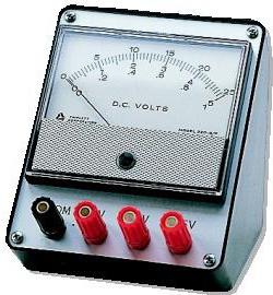
Accuracy of electrical measuring instruments

To specify the accuracy of such devices, a value called the accuracy class is used. For its designation, the letter "Gamma" is used. To accurately determine the absolute and relative measurement errors, you need to know the accuracy class of the device, which is indicated on the scale.

Take, for example, an ammeter. Its scale indicates the accuracy class, which shows the number 0.5. It is suitable for measurements at constant and alternating current, refers to the devices of the electromagnetic system.

This is a fairly accurate device. If you compare it with a school voltmeter, you can see that it has an accuracy class of 4. This value must be known for further calculations.

Application of knowledge

Thus, D c \u003d c (max) X γ / 100

This formula will be used for concrete examples. Let's use a voltmeter and find the error in measuring the voltage that the battery gives.

Let's connect the battery directly to the voltmeter, having previously checked whether the arrow is at zero. When the device was connected, the arrow deviated by 4.2 divisions. This state can be described as follows:

1. It can be seen that the maximum value of U for this subject equals 6.
2. Accuracy class -(γ) = 4.
3. U(o) = 4.2 V.
4. C=0.2 V

Using these formula data, the absolute and relative measurement errors are calculated as follows:

D U \u003d DU (ex.) + C / 2

D U (pr.) \u003d U (max) X γ / 100

D U (pr.) \u003d 6 V X 4/100 \u003d 0.24 V

This is the error of the instrument.

The calculation of the absolute measurement error in this case will be performed as follows:

D U = 0.24 V + 0.1 V = 0.34 V

According to the considered formula, you can easily find out how to calculate absolute error measurements.

There is a rule for rounding errors. It allows you to find average between the limit of absolute error and relative error.

Learning to determine the weighing error

This is one example of direct measurements. On the special place worth weighing. After all, lever scales do not have a scale. Let's learn how to determine the error of such a process. The accuracy of mass measurement is affected by the accuracy of the weights and the perfection of the scales themselves.

We use a balance scale with a set of weights that must be placed exactly on the right side of the scale. Take a ruler for weighing.

Before starting the experiment, you need to balance the scales. We put the ruler on the left bowl.

The mass will be equal to the sum of the installed weights. Let us determine the measurement error of this quantity.

D m = D m (weights) + D m (weights)

The mass measurement error consists of two terms associated with scales and weights. To find out each of these values, at the factories for the production of scales and weights, products are supplied with special documents that allow you to calculate the accuracy.

Application of tables

Let's use a standard table. The error of the scale depends on how much mass is put on the scale. The larger it is, the larger the error, respectively.

Even if you put a very light body, there will be an error. This is due to the process of friction occurring in the axles.

The second table refers to a set of weights. It indicates that each of them has its own mass error. The 10-gram has an error of 1 mg, as well as the 20-gram. We calculate the sum of the errors of each of these weights, taken from the table.

It is convenient to write the mass and the mass error in two lines, which are located one under the other. The smaller the weight, the more accurate the measurement.

Results

In the course of the considered material, it was established that it is impossible to determine the absolute error. You can only set its boundary indicators. For this, the formulas described above in the calculations are used. This material proposed for study at school for students in grades 8-9. Based on the knowledge gained, it is possible to solve problems for determining the absolute and relative errors.